21 Tidyverse
21.1 Acknowledgment/License
The original source for this chapter was from the web site
https://github.com/UoMResearchIT/r-day-workshop/
which was used to build this web page:
https://uomresearchit.github.io/r-day-workshop/04-dplyr/
and is used under the
Attribution 4.0 International (CC BY 4.0)
license https://creativecommons.org/licenses/by/4.0/.
The material presented here has been modified from the original source.
Accordingly this chapter is made available under the same license terms.
21.2 Tidyverse Model for Data Science
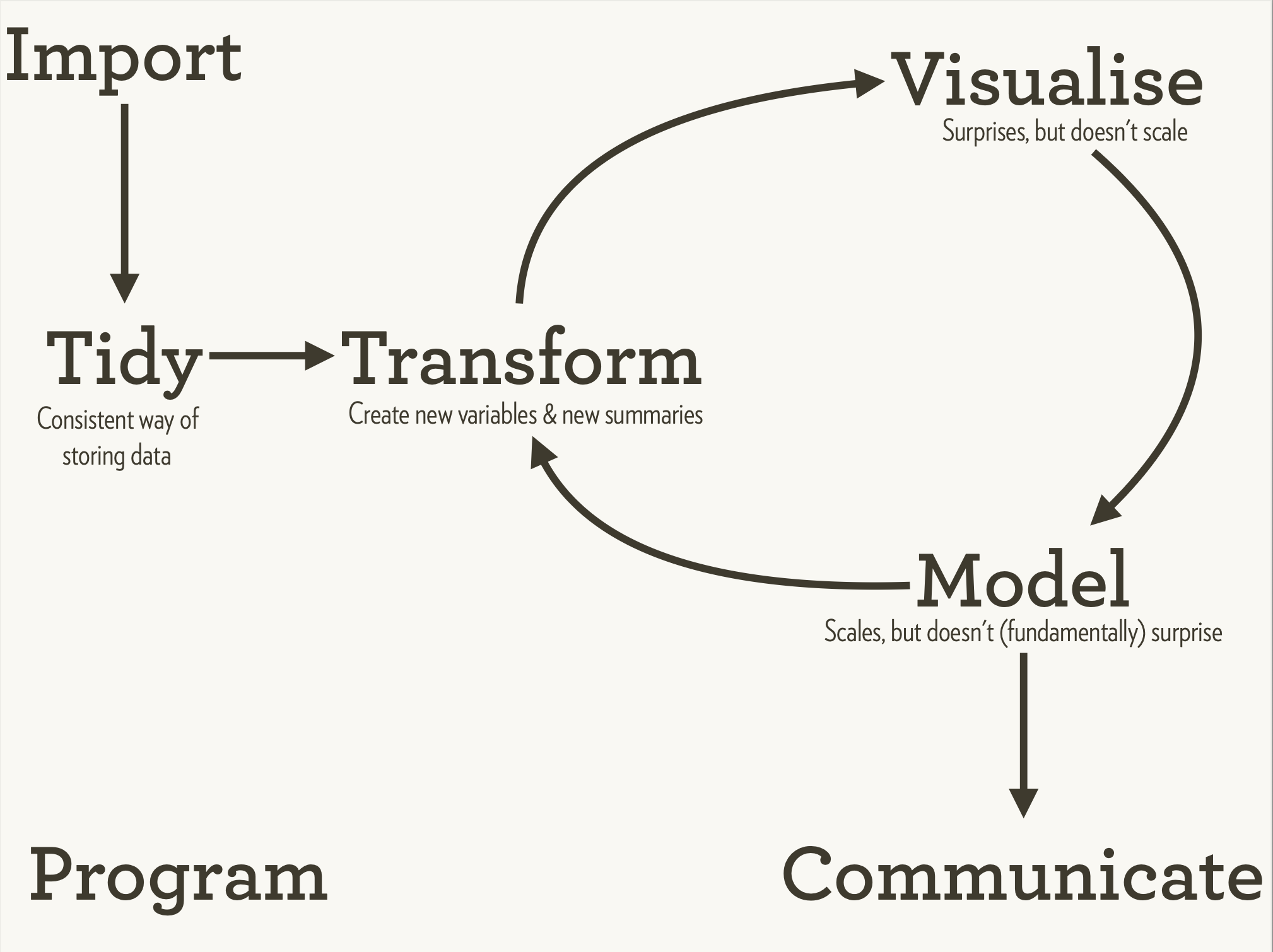
The Tidyverse provides tools for all these aspects of the typical data science workflow:
The Tidyverse aims to make the commands and tools used more consistent with our cognitive approach to data science:
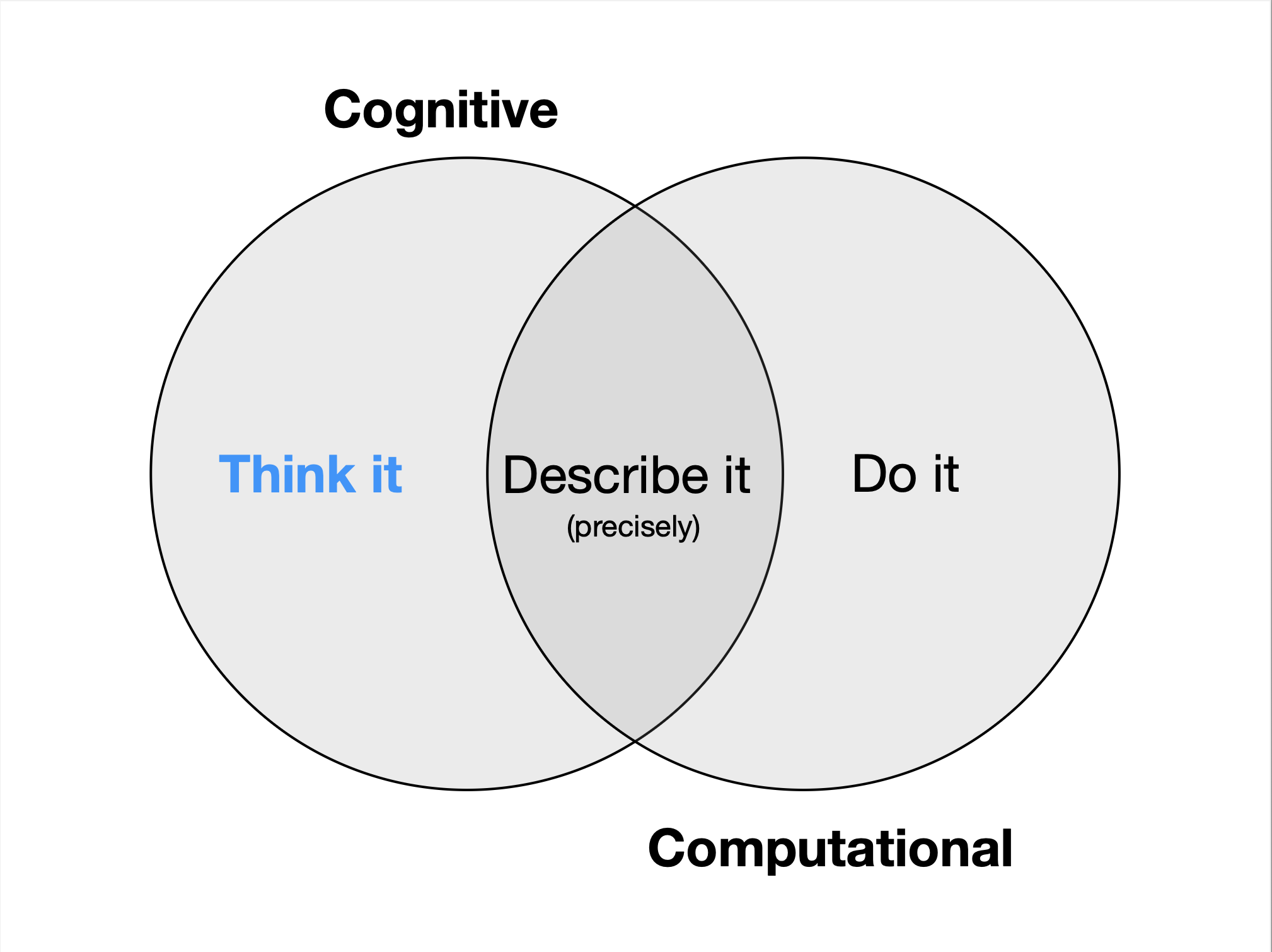
These two images are from slide sets made available by Hadley Wickham, the main creator of the Tidyverse, under the Common Creative Attribution license:

See also
R for Data Science https://r4ds.had.co.nz/explore-intro.html
and
Wickham H, Averick M, Bryan J, Chang W, McGowan LD, François R, Grolemund G, Hayes A, Henry L, Hester J, Kuhn M, Pedersen TL, Miller E, Bache SM, Müller K, Ooms J, Robinson D, Seidel DP, Spinu V, Takahashi K, Vaughan D, Wilke C, Woo K, Yutani H. Welcome to the Tidyverse. Journal of Open Source Software. 2019 Nov 21;4(43):1686. DOI: https://doi.org/10.21105/joss.01686
21.3 Load gapminder data
Let’s use the read_csv() command from the tidyverse package to load gapminder data into a tibble within R.
In this episode we’ll use the dplyr package to manipulate the data we loaded, and calculate some summary statistics. We’ll also introduce the concept of “pipes”.
21.4 Manipulating tibbles
Manipulation of tibbles means many things to many researchers. We often select only certain observations (rows) or variables (columns). We often group the data by a certain variable(s), or calculate summary statistics.
21.5 The dplyr package
The dplyr package is part of the tidyverse. It provides a number of very useful functions for manipulating tibbles (and their base-R cousin, the data.frame) in a way that will reduce repetition, reduce the probability of making errors, and probably even save you some typing.
We will cover:
- selecting variables with
select() - subsetting observations with
filter() - grouping observations with
group_by() - generating summary statistics using
summarize() - generating new variables using
mutate() - Sorting tibbles using
arrange() - chaining operations together using pipes
%>%
21.6 Using select()
If, for example, we wanted to move forward with only a few of the variables in our tibble we use the select() function. This will keep only the variables you select.
Select will select columns of data. What if we want to select rows that meet certain criteria?
21.7 Other ways of selecting
Instead of saying what columns we do want, we can tell R which columns we don’t want by prefixing the column name with a -. For example to select everything except year we would use select(gapminder, -year).
There are also other ways of selecting columns based on parts of their names (such as starts_with() and ends_with()) - see ?select_helpers for more information.
21.8 Using filter()
The filter() function is used to select rows of data. For example, to select only countries in Europe:
Only rows of the data where the condition (i.e. continent=="Europe") is TRUE are kept.
21.9 Using pipes and dplyr
We’ve now seen how to choose certain columns of data (using select()) and certain rows of data (using filter()). In an analysis we often want to do both of these things (and many other things, like calculating summary statistics, which we’ll come to shortly). How do we combine these?
There are several ways of doing this; the method we will learn about today is using pipes.
The pipe operator %>% lets us pipe the output of one command into the next. This allows us to build up a data-processing pipeline. This approach has several advantages:
- We can build the pipeline piecemeal - building the pipeline step-by-step is easier than trying to perform a complex series of operations in one go
- It is easy to modify and reuse the pipeline
- We don’t have to make temporary tibbles as the analysis progresses
Note that R now has a native pipe operator |> which is very similar (but not identical) to the pipe operator %>% used here. The pipe operator %>% is defined by the magrittr R package, which is loaded when we load dplyr or tidyverse.
21.10 Pipelines and the shell
If you’re familiar with the Unix shell, you may already have used pipes to pass the output from one command to the next. The concept is the same, except the shell uses the | character rather than R’s pipe operator %>%
21.11 Keyboard shortcuts and getting help
The pipe operator can be tedious to type. In Rstudio pressing Ctrl + Shift+M under Windows / Linux will insert the pipe operator. On the mac, use ⌘ + Shift+M.
We can use tab completion to complete variable names when entering commands. This saves typing and reduces the risk of error.
RStudio includes a helpful “cheat sheet”, which summarises the main functionality and syntax of dplyr. This can be accessed via the help menu –> cheatsheets –> data transformation with dplyr.
Let’s rewrite the select command example using the pipe operator:
To help you understand why we wrote that in that way, let’s walk through it step by step. First we summon the gapminder tibble and pass it on, using the pipe symbol %>%, to the next step, which is the select() function. In this case we don’t specify which data object we use in the select() function since in gets that from the previous pipe.
What if we wanted to combine this with the filter example? I.e. we want to select year, country and GDP per capita, but only for countries in Europe? We can join these two operations using a pipe; feeding the output of one command directly into the next:
Note that the order of these operations matters; if we reversed the order of the select() and filter() functions, the continent variable wouldn’t exist in the data-set when we came to apply the filter.
What about if we wanted to match more than one item? To do this we use the %in% operator:
21.12 Another way of thinking about pipes
It might be useful to think of the statement
  gapminder %>%
     filter(continent=="Europe") %>%
     select(year,country,gdpPercap)
as a sentence, which we can read as “take the gapminder data and then filter records where continent == Europe and then select the year, country and gdpPercap
We can think of the filter() and select() functions as verbs in the sentence; they do things to the data flowing through the pipeline.
Here’s a nice illustration showing how using pipe syntax results in much easier to understand code:
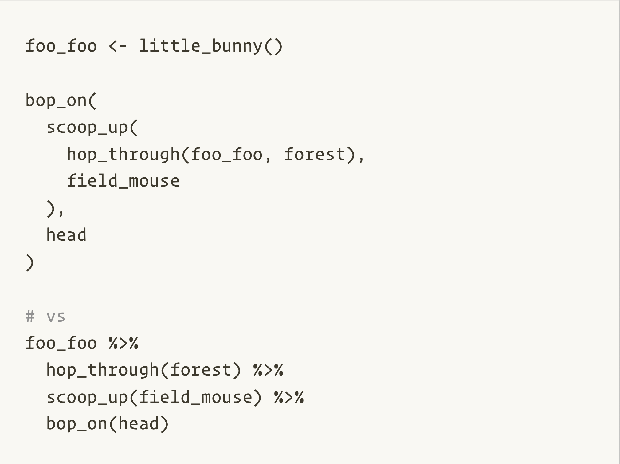
This image is from a slide set made available by Hadley Wickham under the Common Creative Attribution license:
21.13 The dot operator
In the examples above we have passed the output of one command to the next using pipes. The output of one command becomes the first argument of the next command.
This is the default behaviour of pipes. If we want to pass the output of one command to a different argument of the next command, we can use the dot operator . to indicate where the output should go. For example, if we wanted to filter the gapminder data to only include rows where the year is 2007, we could do this:
Here the first dot operator . indicates that the output of the previous command should be used as the data frame to be filtered. The second dot operator .$year indicates that we want to use the year variable from that same data frame.
Note also that this is equivalent to the following, where we have used the dot operator in every part of the pipeline:
This is a reminder that the majority of Tidyverse functions take a data frame as their first argument, so that in a pipeline the output of one command can be automatically assigned the first argument of the next command. However, this is more verbose than necessary, so we usually omit the dot operator when it is not needed.
It also illustrates that we can use base R filtering/subsetting within a pipeline and we can include other base R functions (like head()) within a pipeline.
21.14 Splitting your commands over multiple lines
It’s generally a good idea to put one command per line when writing your analyses. This makes them easier to read. When doing this, it’s important that the %>% goes at the end of the line, as in the example above. If we put it at the beginning of a line, e.g.:
the first line makes a valid R command. R will then treat the next line as a new command, which won’t work.
Write a single command (which can span multiple lines and includes pipes) that will produce a tibble that has the values of lifeExp, country and year, for the countries in Africa, but not for other Continents. How many rows does your tibble have? (You can use the nrow() function to find out how many rows are in a tibble.)
As with last time, first we pass the gapminder tibble to the filter() function, then we pass the filtered version of the gapminder tibble to the select() function. Note: The order of operations is very important in this case. If we used ‘select’ first, filter would not be able to find the variable continent since we would have removed it in the previous step.
21.15 Sorting tibbles
The arrange() function will sort a tibble by one or more of the variables in it:
We can use the desc() function to sort a variable in reverse order:
21.16 Generating new variables
The mutate() function lets us add new variables to our tibble. It will often be the case that these are variables we derive from existing variables in the data-frame.
As an example, the gapminder data contains the population of each country, and its GDP per capita. We can use this to calculate the total GDP of each country:
We can also use functions within mutate to generate new variables. For example, to take the log of gdpPercap we could use:
The dplyr cheat sheet contains many useful functions which can be used with dplyr. This can be found in the help menu of RStudio. You will use one of these functions in the next challenge.
Create a tibble containing each country in Europe, its life expectancy in 2007 and the rank of the country’s life expectancy. (note that ranking the countries will not sort the table; the row order will be unchanged. You can use the arrange() function to sort the table).
Hint: First filter() to get the rows you want, and then use mutate() to create a new variable with the rank in it. The cheat-sheet contains useful functions you can use when you make new variables (the cheat-sheets can be found in the help menu in RStudio).
There are several functions for ranking observations, which handle tied values differently (including rank, min_rank, and dense_rank). For this exercise it doesn’t matter which function you choose.
Can you reverse the ranking order so that the country with the longest life expectancy gets the lowest rank? Hint: This is similar to sorting in reverse order
To reverse the order of the ranking, use the desc function, i.e. mutate(rank = min_rank(desc(lifeExp)))
There are several functions for calculating ranks; you may have used, e.g. dense_rank() The min_rank and dense_rank functions handle ties differently. The help file for dplyr’s ranking functions explains the differences, and can be accessed with ?dense_rank or ?min_rank.
21.17 Calculating summary statistics
We often wish to calculate a summary statistic (the mean, standard deviation, etc.) for a variable. We frequently want to calculate a separate summary statistic for several groups of data (e.g. the experiment and control group). We can calculate a summary statistic for the whole data-set using the dplyr’s summarise() function:
To generate summary statistics for each value of another variable we use the group_by() function:
21.18 Aside
In the examples above it would be preferable to calculate the weighted mean (to reflect the different populations of the countries). R can calculate this for us using weighted.mean(lifeExp, pop). For simplicty we’ve used the regular mean in the above examples.
For each combination of continent and year, calculate the average life expectancy.
21.19 count() and n()
A very common operation is to count the number of observations for each group. The dplyr package comes with two related functions that help with this.
If we need to use the number of observations in calculations, the n() function is useful. For instance, if we wanted to get the standard error of the life expectancy per continent:
Although we could use the group_by(), n() and summarize() functions to calculate the number of observations in each group, dplyr provides the count() function which automatically groups the data, calculates the totals and then ungroups it.
For instance, if we wanted to check the number of countries included in the dataset for the year 2002, we can use:
We can optionally sort the results in descending order by adding sort=TRUE:
21.20 Equivalent functions in base R
In this chapter we’ve taught the tidyverse. You are likely come across code written others in base R.
21.21 Other great resources
- Data Wrangling tutorial - an excellent four part tutorial covering selecting data, filtering data, summarising and transforming your data.
- R for Data Science
- “Data Transformation with dplyr” cheatset available in RStudio via Help -> Cheat Sheets
- Introduction to dplyr - this is the package vignette. It can be viewed within R using
vignette(package="dplyr", "dplyr")