Mentorship
Daniel E. Weeks November 21, 2020, 14:11
- 1 Load Libraries
- 2 Input directory and files
- 3 The AlShebli et al (2020) mentorship paper
- 4 The data
- 5 ProtegeFirstPubYear
- 6 Distribution of ProtegeFirstPubYear
- 7 NumYearsPostMentorship
- 8 AvgMentorsAcAges
- 9 Avg_c5
- 10 Avg_c10
- 11 Avg_c5 vs Avg_c10
- 12 numMentors
- 13 Summary
- 13.1 Problem: No gender information for mentors
- 13.2 Problem: ProtegeFirstPubYear time range is very large
- 13.3 Problem: Error in the equation for NumYearsPostMentorship
- 13.4 Problem: some values of
NumYearsPostMentorshipare unrealistically large - 13.5 Problem: some
AvgMentorsAcAgesare unrealistically large - 13.6 Problem with Avg_c10: Cannot compute a value
Avg_c10for recent publications - 13.7 Problem: some
numMentorsvalues are too large
- 14 Generating GitHub Markdown
- 15 Session Information
1 Load Libraries
library(tidyverse)
# library(tidylog)
library(ggExtra)
library(arsenal)
2 Input directory and files
# Print the working directory
getwd()
## [1] "/Users/dweeks/data/Mentorship"
3 The AlShebli et al (2020) mentorship paper
Here I examine the data provided by the authors of this paper:
AlShebli B, Makovi K, Rahwan T. The association between early career informal mentorship in academic collaborations and junior author performance. Nat Commun. 2020 Nov 17;11(1):5855. doi: 10.1038/s41467-020-19723-8. PMID: 33203848. https://pubmed.ncbi.nlm.nih.gov/33203848/
4 The data
4.1 The input data
The input data are from the ‘bedoor/Mentorship’ GitHub repository at
https://github.com/bedoor/Mentorship
Their repository is described as:
‘This repository includes all data used in “The Association between Early Career Informal Mentorship in Academic Collaborations and Junior Author Performance”.’
LinesRead <- 1e+05
inFile <- "Mentorship/Repository_Data/Data_7yearcutoff.csv"
a <- read_csv(file = inFile, n_max = LinesRead)
## Parsed with column specification:
## cols(
##   .default = col_double(),
##   Pr0tegeGender = col_character(),
##   AffiliationRank = col_character()
## )

## See spec(...) for full column specifications.
names(a)
##  [1] "Disambiguated_ProtegeID"   "AvgBigShot"
##  [3] "AvgBigShotBin"             "AvgHub"
##  [5] "AvgHubBin"                 "Avg_c5"
##  [7] "numMentors"                "numMentorsBin"
##  [9] "ProtegeFirstPubYear"       "ProtegeFirstPubYearBin"
## [11] "Pr0tegeGender"             "ProtegeGenderBin"
## [13] "AffiliationRank"           "AffiliationRankBin"
## [15] "AvgMentorsAcAges"          "AvgMentorsAcAgesBin"
## [17] "NumYearsPostMentorship"    "NumYearsPostMentorshipBin"
## [19] "ProtegeDisciplineID"       "Avg_c10"
## [21] "MaxBigShot"                "MaxBigShotBin"
## [23] "MedianBigShot"             "MedianBigShotBin"
## [25] "MaxHub"                    "MaxHubBin"
## [27] "MedianHub"                 "MedianHubBin"
total_records <- as.integer(system2("wc", args = c("-l", inFile, " | awk '{print $1}'"),
    stdout = TRUE))
total_records
## [1] 1055213
4.2 Disclaimer: For speed, only read in the first 10^{5} lines
To speed up the analyses, we read only the first 10^{5} lines of the input file, instead of reading all 1055213 lines.
4.3 Problem: No gender information for mentors
There does not appear to be any information in the provided file about the mentor’s gender, so the provided data do not appear to be ‘all the data’.
There is no data dictionary, so we are left to infer what is in each column of the data file from the column names and content.
5 ProtegeFirstPubYear
6 Distribution of ProtegeFirstPubYear
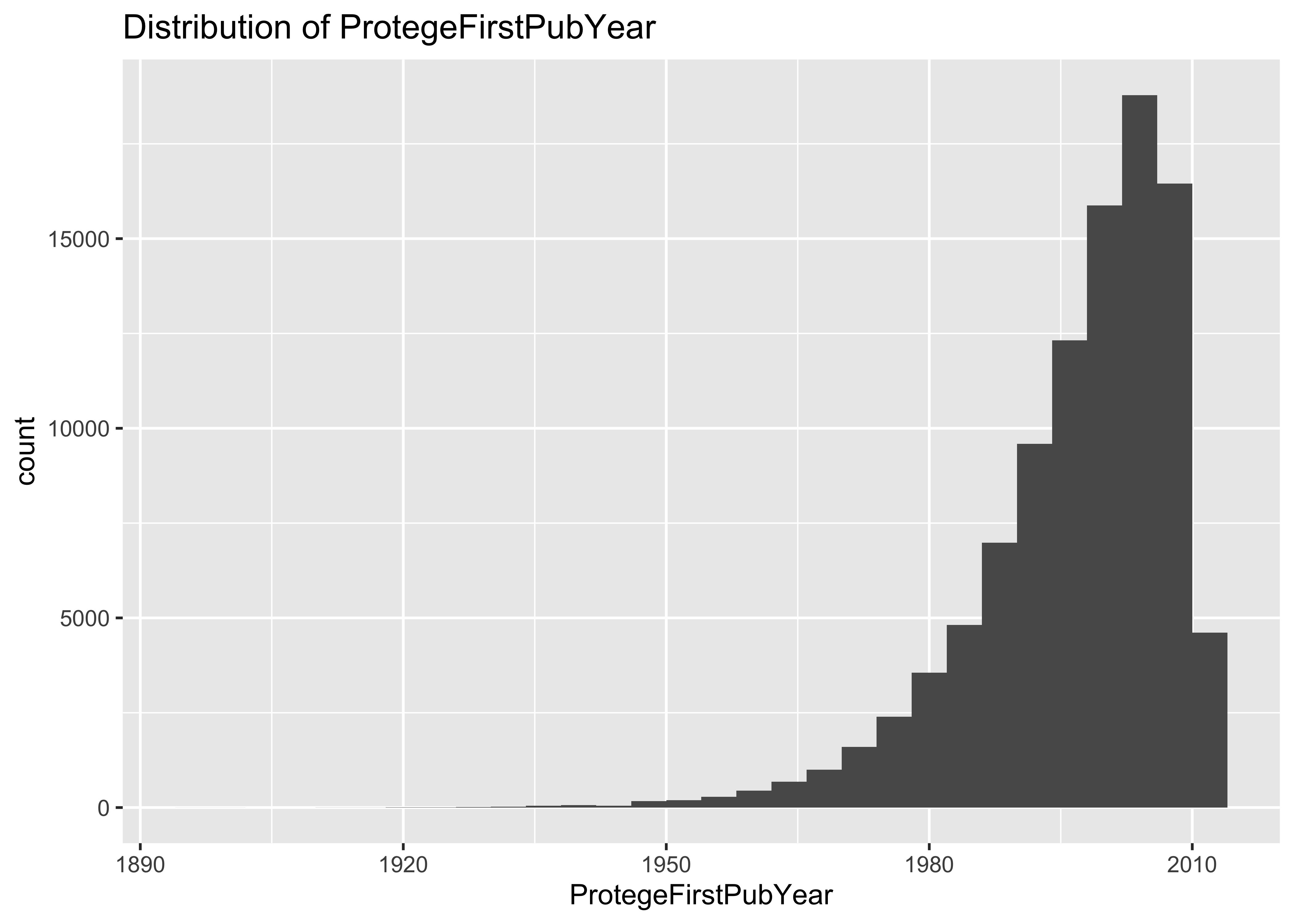
“Year of the protege’s first publication: The year in which the protege published their first mentored paper.”
summary(a$ProtegeFirstPubYear)
##    Min. 1st Qu.  Median    Mean 3rd Qu.    Max.
##    1897    1992    2000    1997    2006    2013
ggplot(data = a, mapping = aes(x = ProtegeFirstPubYear)) + geom_histogram() + ggtitle("Distribution of ProtegeFirstPubYear")
## `stat_bin()` using `bins = 30`. Pick better value with `binwidth`.
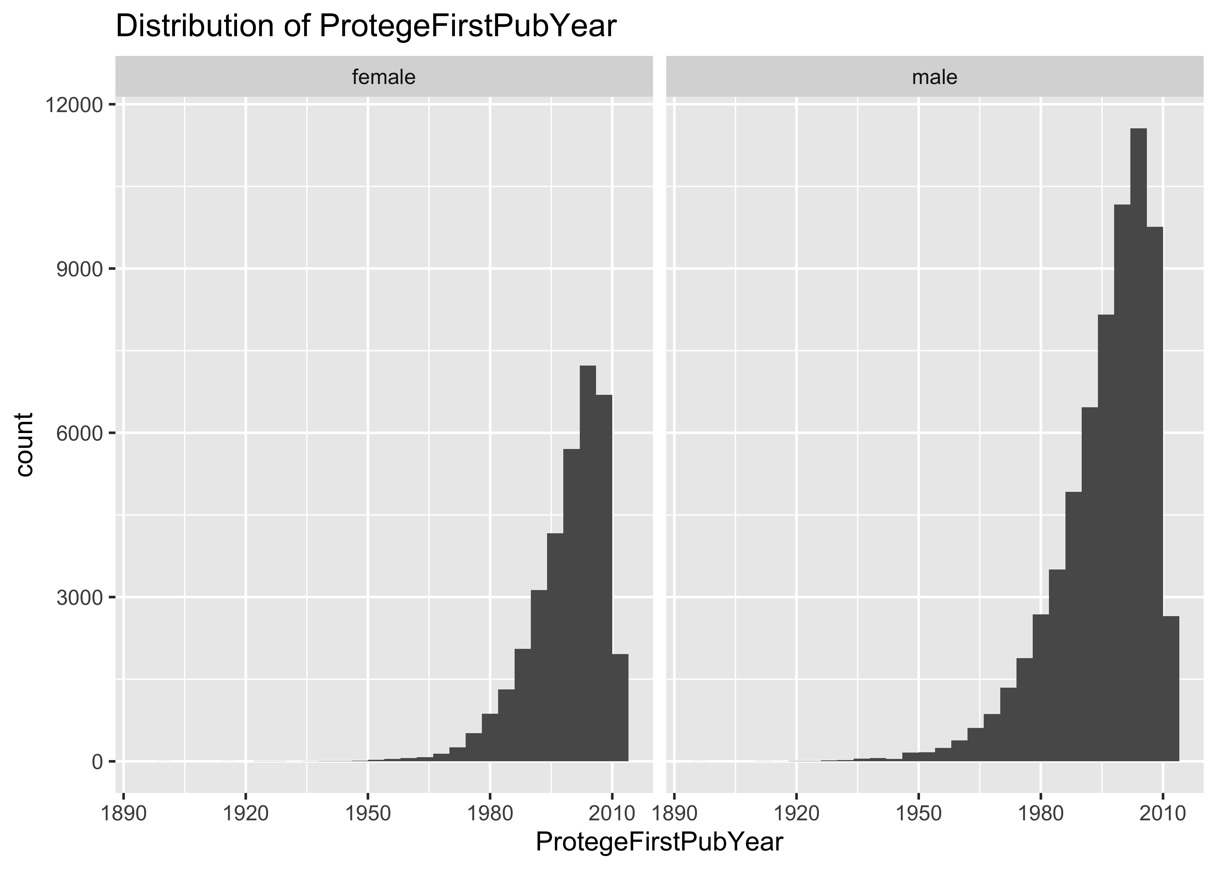
table(a$Pr0tegeGender)
##
## female   male
##  34257  65743
ggplot(data = a, mapping = aes(x = ProtegeFirstPubYear)) + geom_histogram() + ggtitle("Distribution of ProtegeFirstPubYear") +
    facet_grid(~Pr0tegeGender)
## `stat_bin()` using `bins = 30`. Pick better value with `binwidth`.
a$MaleProtegeFirstPubYear <- a$ProtegeFirstPubYear
a$MaleProtegeFirstPubYear[a$Pr0tegeGender == "female"] <- NA
a$FemaleProtegeFirstPubYear <- a$ProtegeFirstPubYear
a$FemaleProtegeFirstPubYear[a$Pr0tegeGender == "male"] <- NA
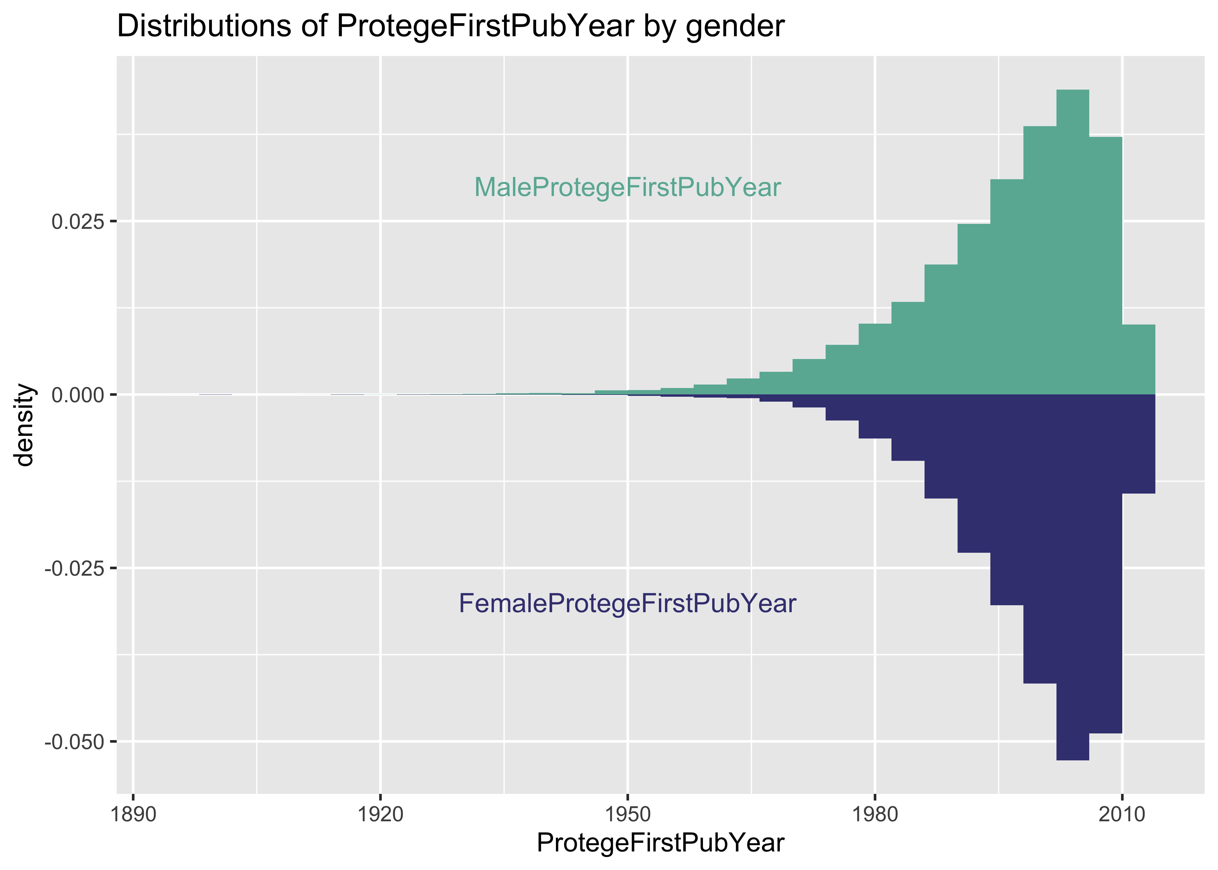
summary(a$MaleProtegeFirstPubYear)
##    Min. 1st Qu.  Median    Mean 3rd Qu.    Max.    NA's
##    1897    1990    1999    1996    2005    2013   34257
summary(a$FemaleProtegeFirstPubYear)
##    Min. 1st Qu.  Median    Mean 3rd Qu.    Max.    NA's
##    1901    1995    2002    2000    2007    2013   65743
p <- ggplot(data = a, aes(x = x)) + geom_histogram(aes(x = MaleProtegeFirstPubYear,
    y = ..density..), fill = "#69b3a2") + annotate("text", x = 1950, y = 0.03, label = "MaleProtegeFirstPubYear",
    color = "#69b3a2") + geom_histogram(aes(x = FemaleProtegeFirstPubYear, y = -..density..),
    fill = "#404080") + annotate("text", x = 1950, y = -0.03, label = "FemaleProtegeFirstPubYear",
    color = "#404080") + xlab("ProtegeFirstPubYear") + ggtitle("Distributions of ProtegeFirstPubYear by gender")
p
## `stat_bin()` using `bins = 30`. Pick better value with `binwidth`.

## Warning: Removed 34257 rows containing non-finite values (stat_bin).

## `stat_bin()` using `bins = 30`. Pick better value with `binwidth`.

## Warning: Removed 65743 rows containing non-finite values (stat_bin).
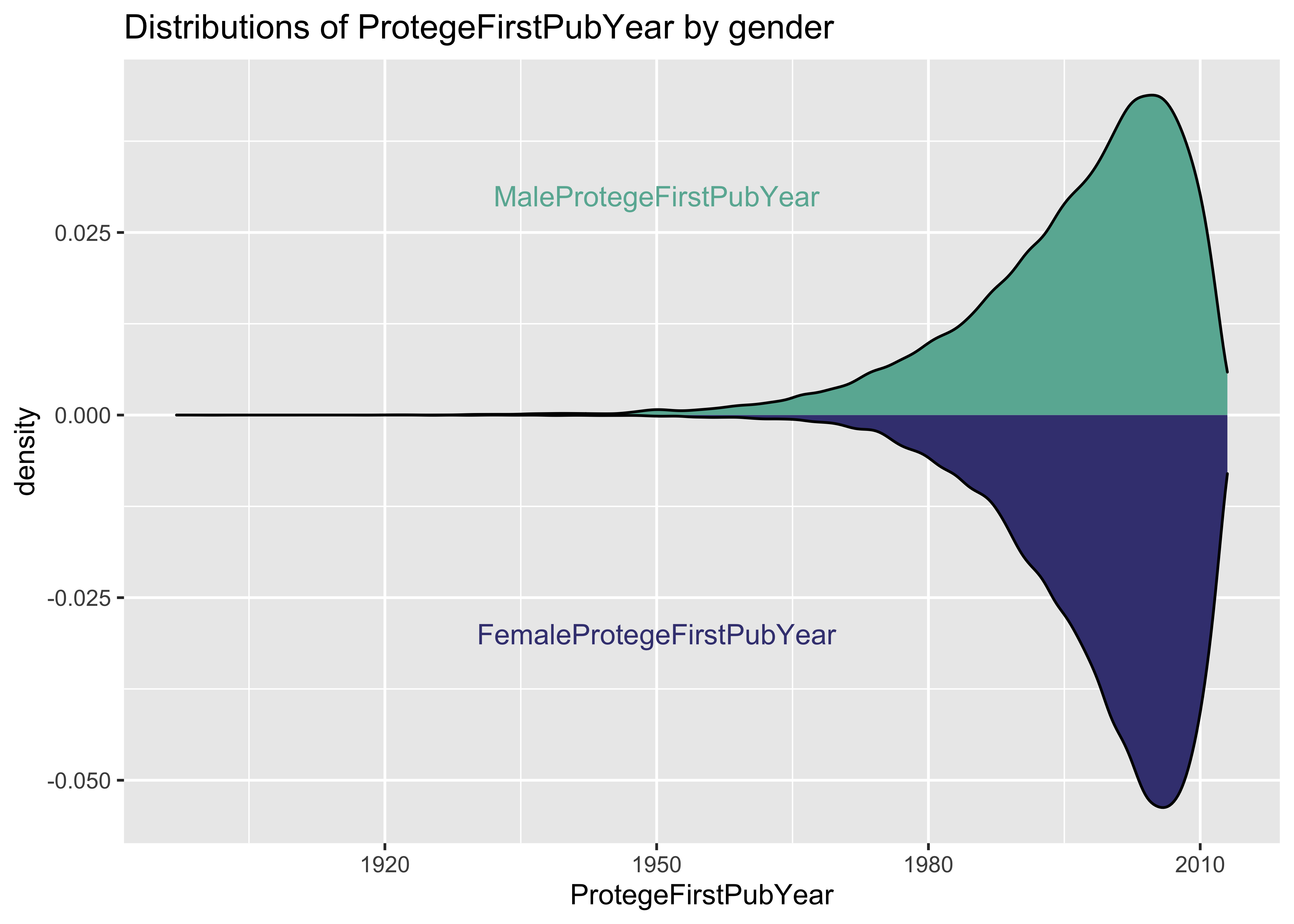
p <- ggplot(data = a, aes(x = x)) + geom_density(aes(x = MaleProtegeFirstPubYear,
    y = ..density..), fill = "#69b3a2") + annotate("text", x = 1950, y = 0.03, label = "MaleProtegeFirstPubYear",
    color = "#69b3a2") + geom_density(aes(x = FemaleProtegeFirstPubYear, y = -..density..),
    fill = "#404080") + annotate("text", x = 1950, y = -0.03, label = "FemaleProtegeFirstPubYear",
    color = "#404080") + xlab("ProtegeFirstPubYear") + ggtitle("Distributions of ProtegeFirstPubYear by gender")
p
## Warning: Removed 34257 rows containing non-finite values
## (stat_density).

## Warning: Removed 65743 rows containing non-finite values
## (stat_density).
6.1 Problem: ProtegeFirstPubYear time range is very large
in the first 10^{5} lines of this data set, the ProtegeFirstPubYear
ranges from 1897 to 2013. It seems that it would be very difficult to
properly compare the impact factors of papers published in
rmin(a$ProtegeFirstPubYear)`, well before the advent of team science
and the current deluge of scientific publications, to those published as
recently 2013.
7 NumYearsPostMentorship
“The number of years post mentorship: Since our dataset is up to Dec 31st 2019, we are only able to calculate c5—the number of citations accumulated five years post publication—for papers published before
- Thus, given a protege whose first paper was published in year x,
the number of years post mentorship is
2015 - (x + 6), bearing in mind that the mentorship period is 7 years and we do not include proteges with a gap of 5 years of more in their career history.”
7.1 Problem: Error in the equation for NumYearsPostMentorship
Note that the stated equation of 2015 - (x + 6) for computing the
number of years post mentorship is not what was used, as instead
2015 - (x + 2), where x is the year the protege’s paper was first
published, as we see here in the first 10^{5} lines of the input file:
all.equal(a$NumYearsPostMentorship, 2015 - (a$ProtegeFirstPubYear + 2))
## [1] TRUE
7.2 Distribution of NumYearsPostMentorship
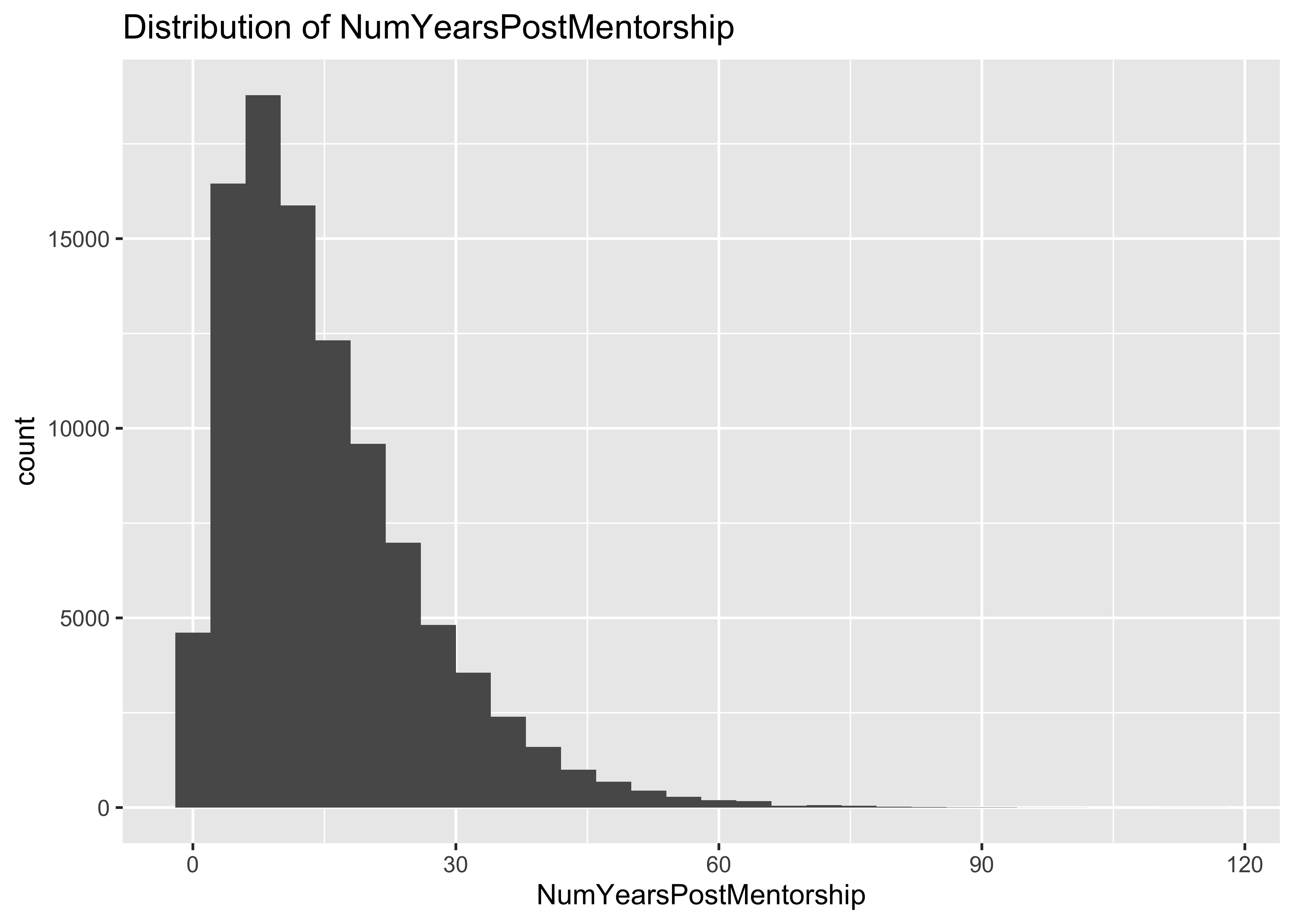
summary(a$NumYearsPostMentorship)
##    Min. 1st Qu.  Median    Mean 3rd Qu.    Max.
##    0.00    7.00   13.00   15.68   21.00  116.00
ggplot(data = a, mapping = aes(x = NumYearsPostMentorship)) + geom_histogram() +
    ggtitle("Distribution of NumYearsPostMentorship")
## `stat_bin()` using `bins = 30`. Pick better value with `binwidth`.
a$ProtegeGender <- as.factor(a$Pr0tegeGender)
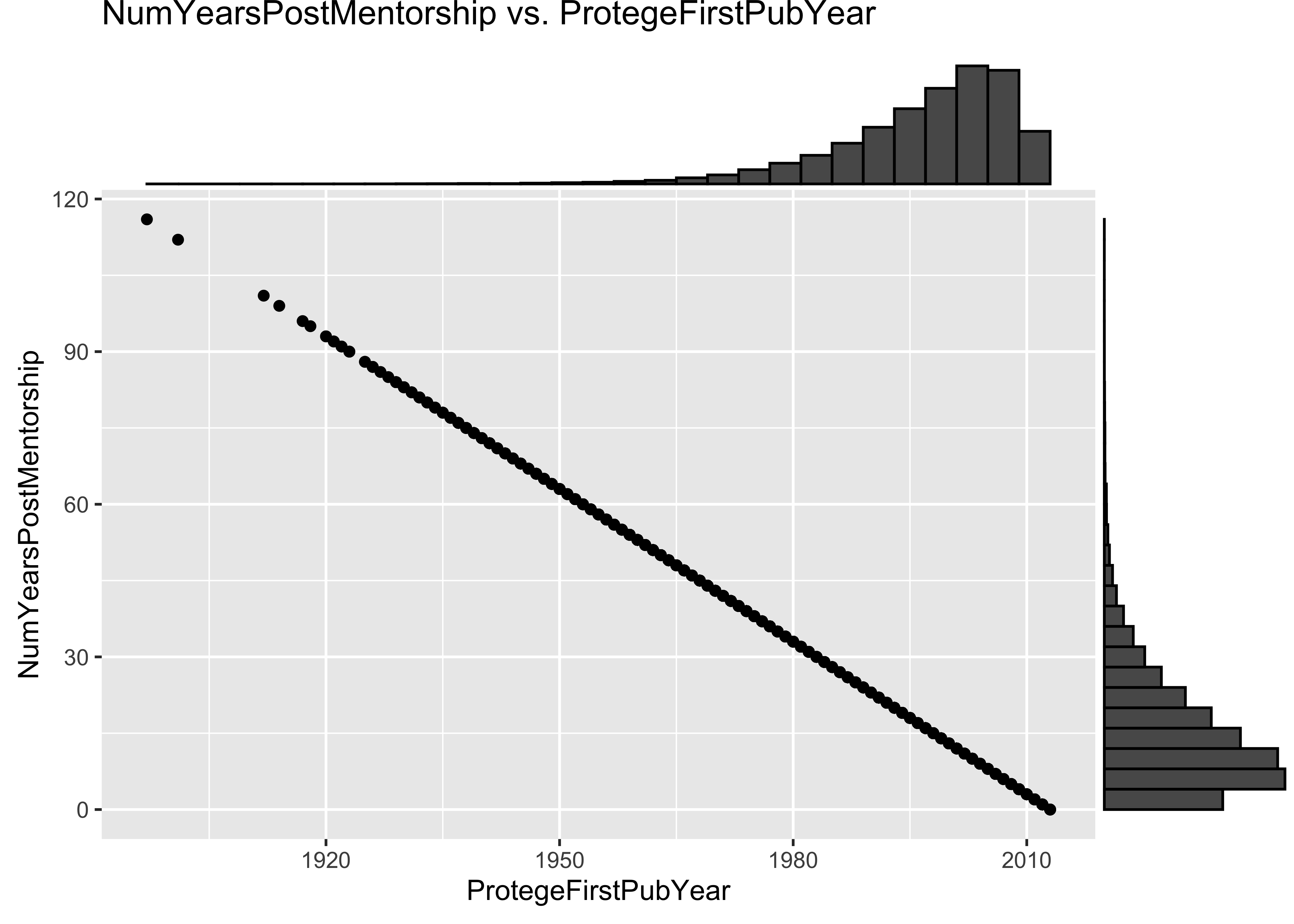
p <- ggplot(data = a, mapping = aes(x = ProtegeFirstPubYear, y = NumYearsPostMentorship)) +
geom_point() + ggtitle("NumYearsPostMentorship vs. ProtegeFirstPubYear")
ggMarginal(p, type = "histogram")

7.3 Problem: some values of NumYearsPostMentorship are unrealistically large
In the first 10^{5} lines of the input file of this data set, there are
values of NumYearsPostMentorship as large as 116. These values are
unrealistically large.
8 AvgMentorsAcAges
8.1 Distribution of AvgMentorsAcAges
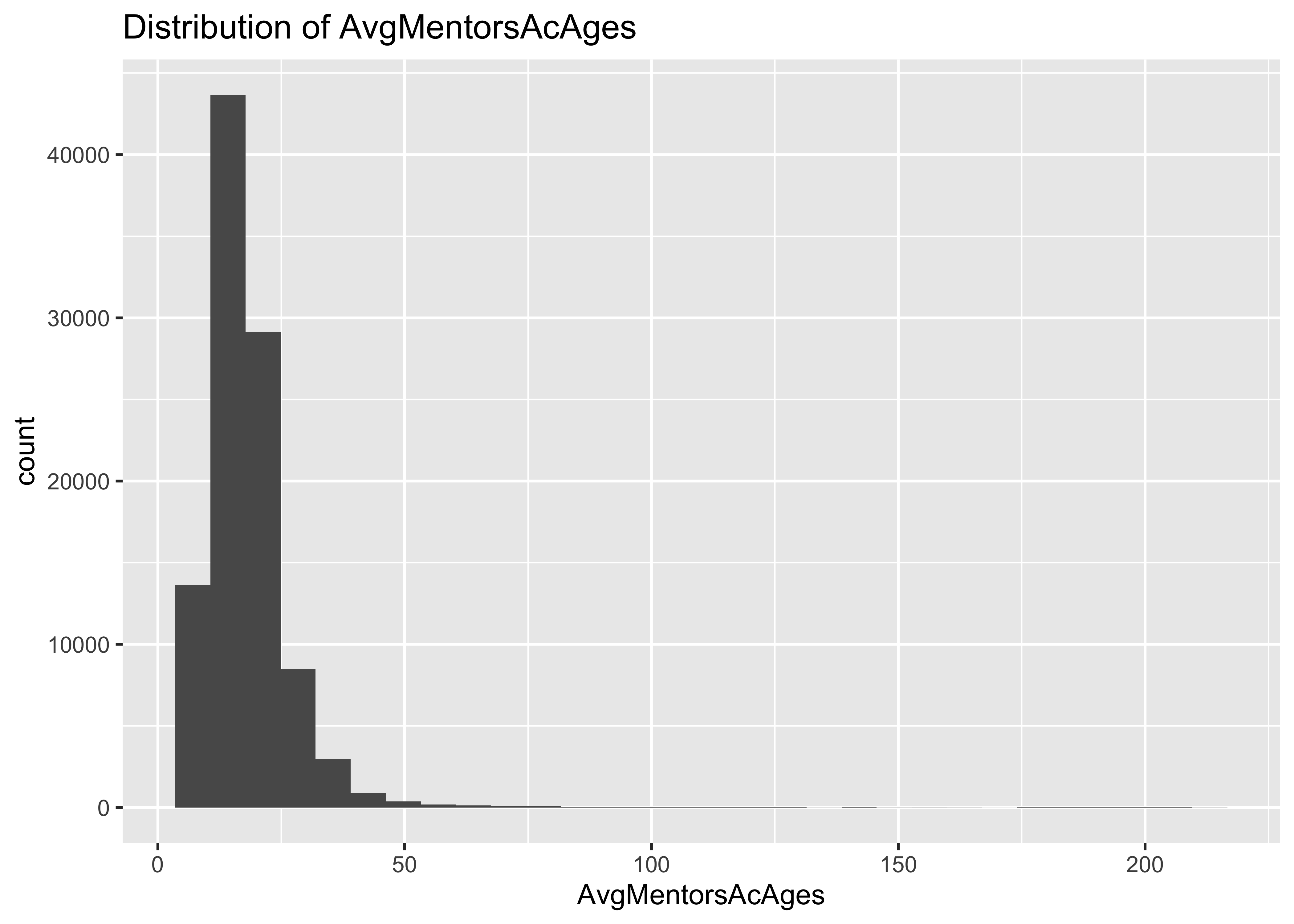
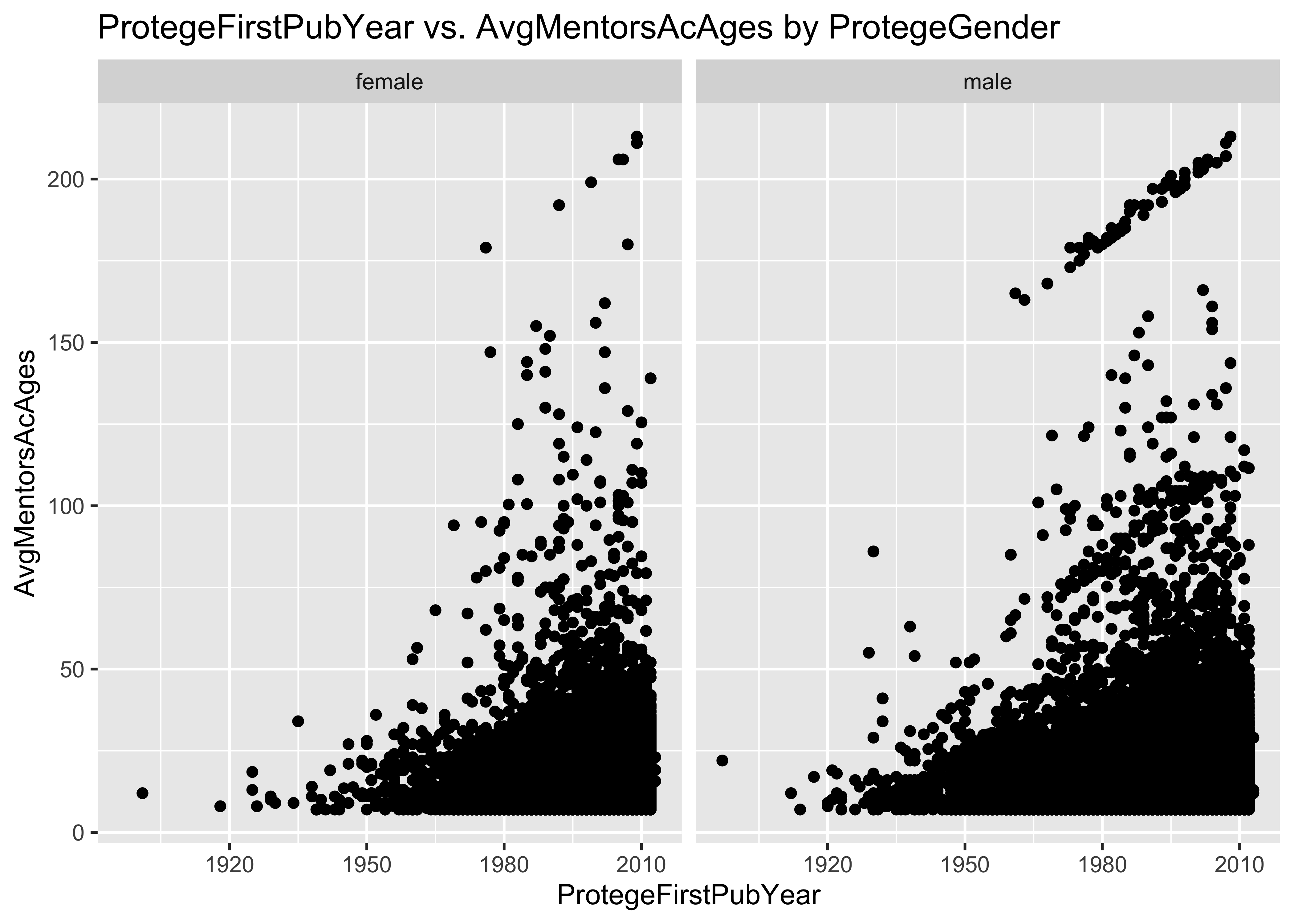
“Average academic age of mentors: This is computed for any given protege by first computing the academic age of each mentor in the year of their first publication with the protege, and then averaging these numbers over all the mentors.”
“Given a scientist whose first paper was published in year x, the academic age of this scientist in year y is y-x.”
summary(a$AvgMentorsAcAges)
##    Min. 1st Qu.  Median    Mean 3rd Qu.    Max.
##    7.00   13.00   16.67   18.18   21.00  213.00
ggplot(data = a, mapping = aes(x = AvgMentorsAcAges)) + geom_histogram() + ggtitle("Distribution of AvgMentorsAcAges")
## `stat_bin()` using `bins = 30`. Pick better value with `binwidth`.
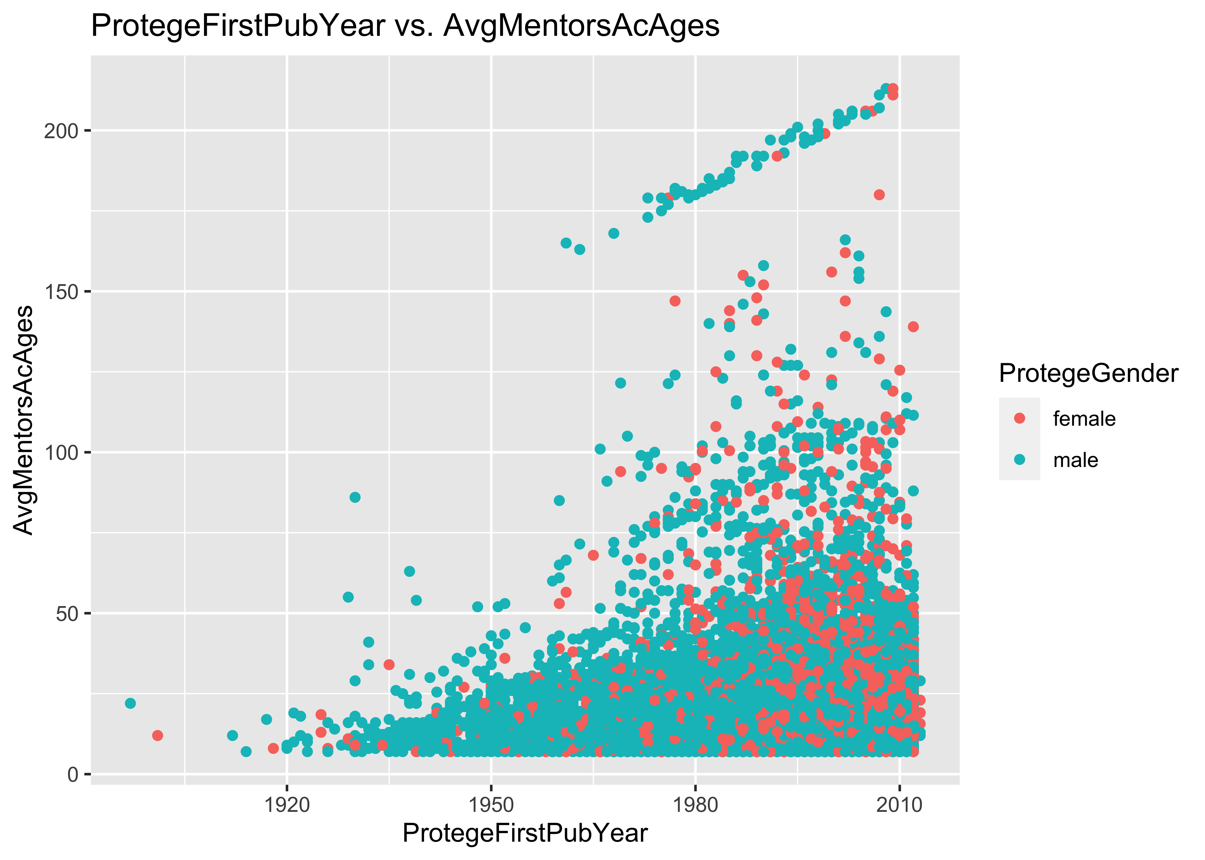
ggplot(data = a, mapping = aes(x = ProtegeFirstPubYear, y = AvgMentorsAcAges, col = ProtegeGender)) +
    geom_point() + ggtitle("ProtegeFirstPubYear vs. AvgMentorsAcAges")
ggplot(data = a, mapping = aes(x = ProtegeFirstPubYear, y = AvgMentorsAcAges)) +
    geom_point() + facet_grid(~ProtegeGender) + ggtitle("ProtegeFirstPubYear vs. AvgMentorsAcAges by ProtegeGender")

8.2 Problem: some AvgMentorsAcAges are unrealistically large
There are AvgMentorsAcAges as large as 213 in the first 10^{5} lines
of this data set. This is unrealistically large.
Among proteges who published their first paper after 2000, there are
AvgMentorsAcAges as large as 213 in this data set. Should we be
evaluating the mentorship effects of mentors who were born than 200
years ago?
9 Avg_c5
9.1 Distribution of Avg_c5
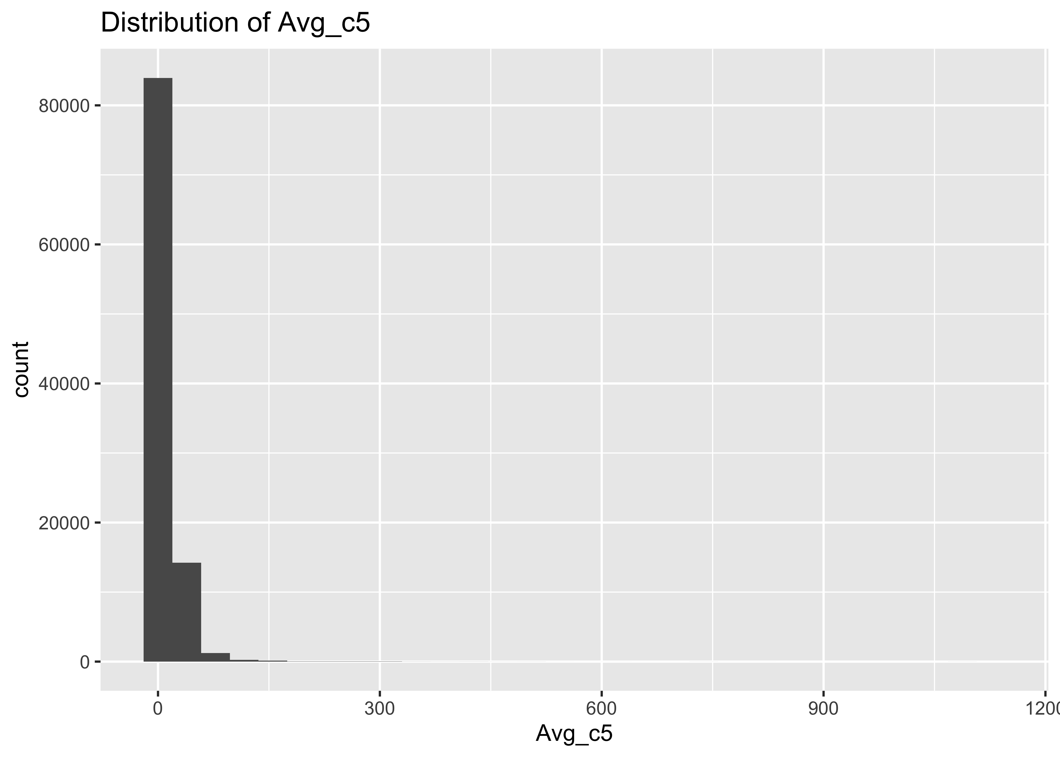
summary(a$Avg_c5)
##     Min.  1st Qu.   Median     Mean  3rd Qu.     Max.
##    0.000    2.068    6.692   11.557   14.254 1126.429
ggplot(data = a, mapping = aes(x = Avg_c5)) + geom_histogram() + ggtitle("Distribution of Avg_c5")
## `stat_bin()` using `bins = 30`. Pick better value with `binwidth`.
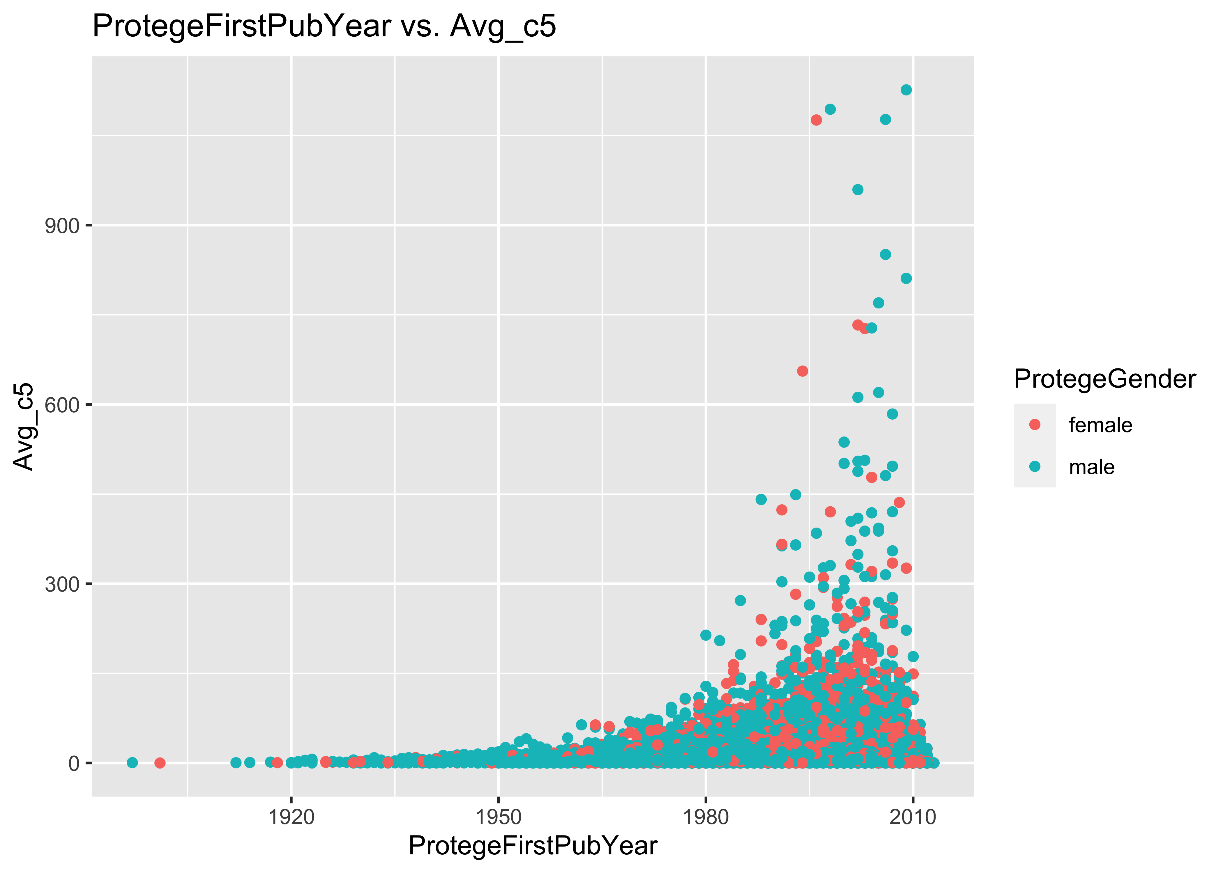
ggplot(data = a, mapping = aes(x = ProtegeFirstPubYear, y = Avg_c5, col = ProtegeGender)) +
    geom_point() + ggtitle("ProtegeFirstPubYear vs. Avg_c5")
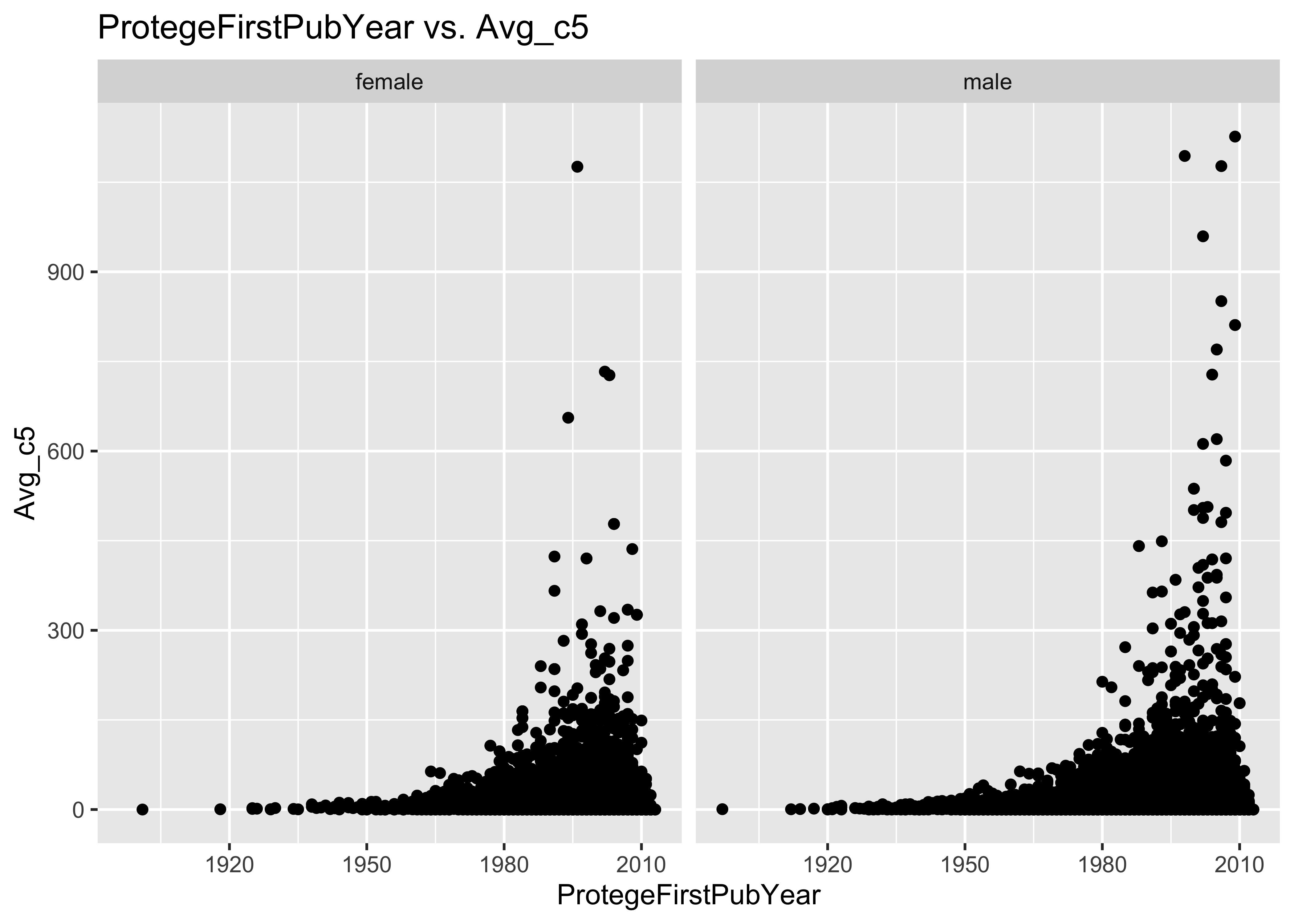
ggplot(data = a, mapping = aes(x = ProtegeFirstPubYear, y = Avg_c5)) + geom_point() +
    facet_grid(~ProtegeGender) + ggtitle("ProtegeFirstPubYear vs. Avg_c5")
9.2 Joint distribution of Avg_c5 and AvgMentorsAcAges
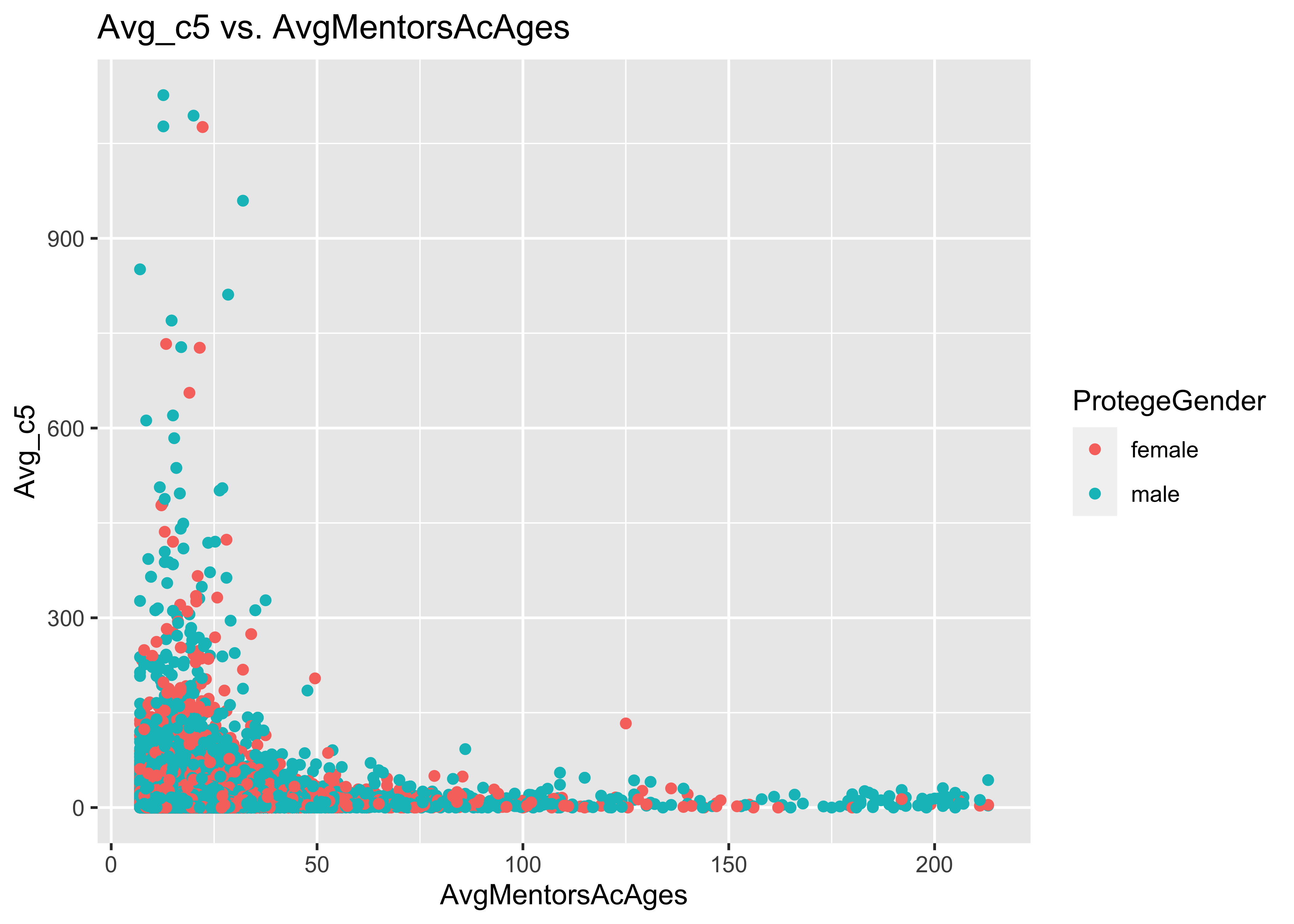
ggplot(data = a, mapping = aes(y = Avg_c5, x = AvgMentorsAcAges, col = ProtegeGender)) +
    geom_point() + ggtitle("Avg_c5 vs. AvgMentorsAcAges")
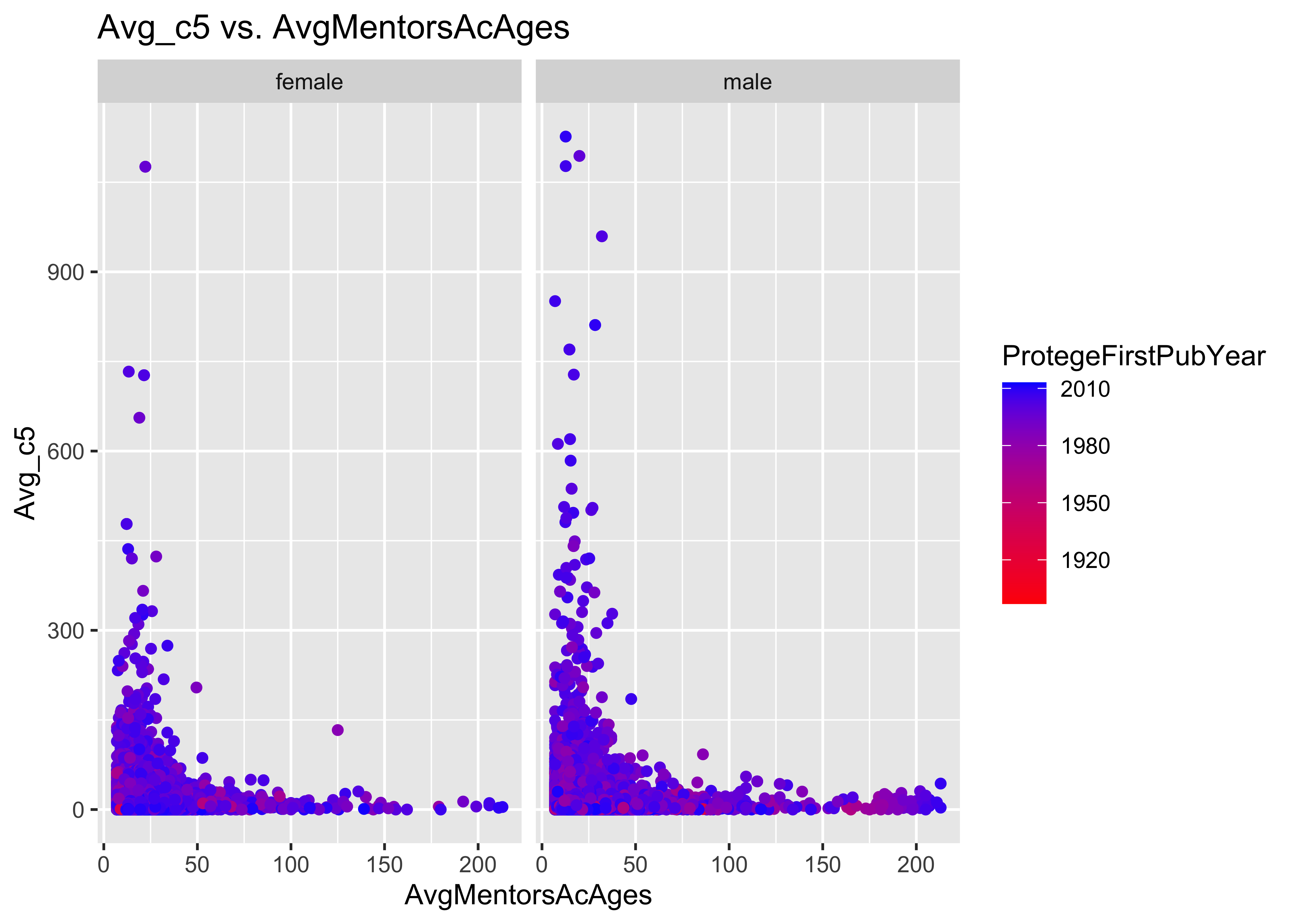
ggplot(data = a, mapping = aes(y = Avg_c5, x = AvgMentorsAcAges, col = ProtegeFirstPubYear)) +
    geom_point() + scale_color_gradient(low = "red", high = "blue") + facet_grid(~ProtegeGender) +
    ggtitle("Avg_c5 vs. AvgMentorsAcAges")
10 Avg_c10
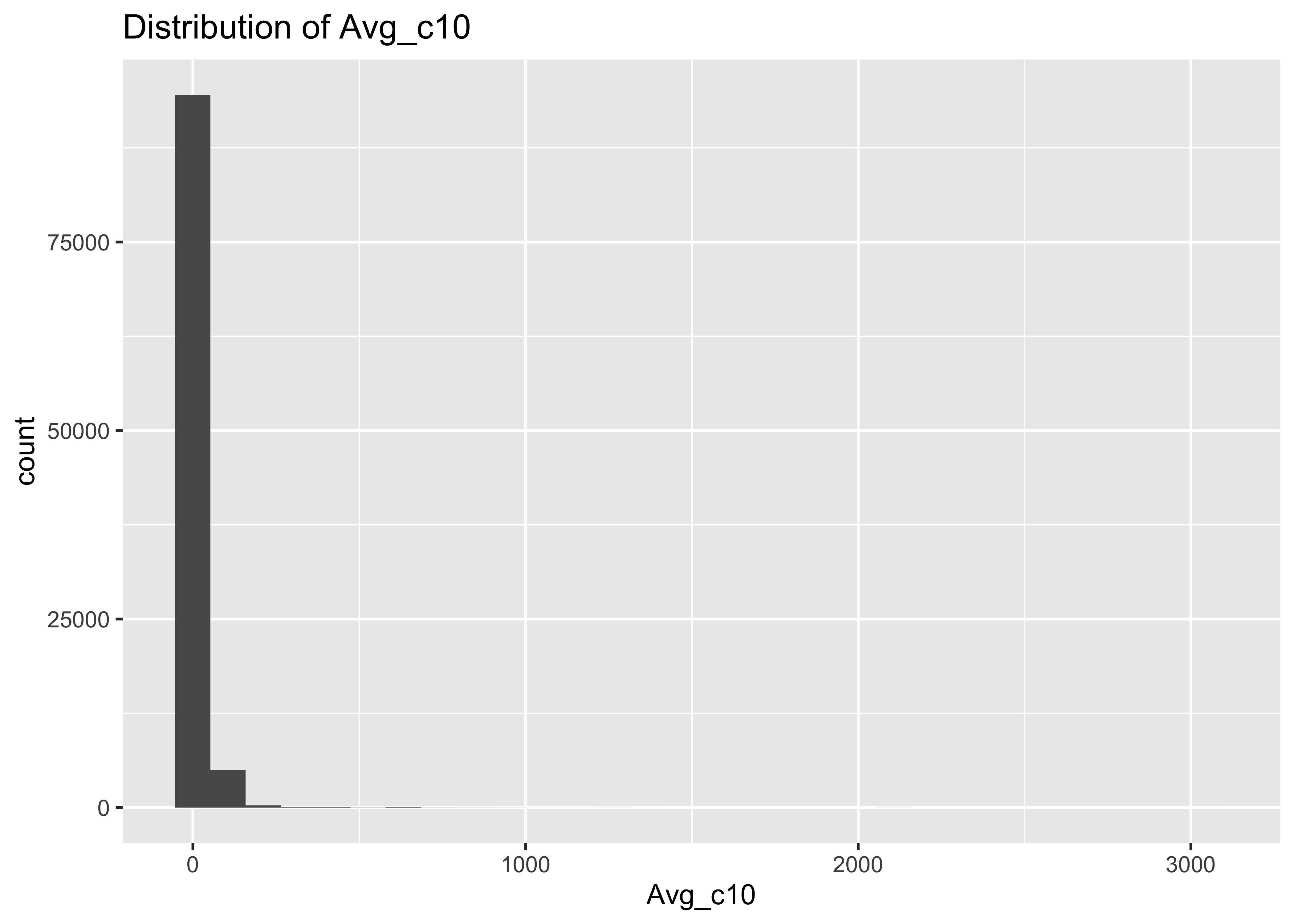
10.1 Distribution of Avg_c10
summary(a$Avg_c10)
##     Min.  1st Qu.   Median     Mean  3rd Qu.     Max.
##    0.000    2.694    9.093   16.945   20.857 3057.000
ggplot(data = a, mapping = aes(x = Avg_c10)) + geom_histogram() + ggtitle("Distribution of Avg_c10")
## `stat_bin()` using `bins = 30`. Pick better value with `binwidth`.
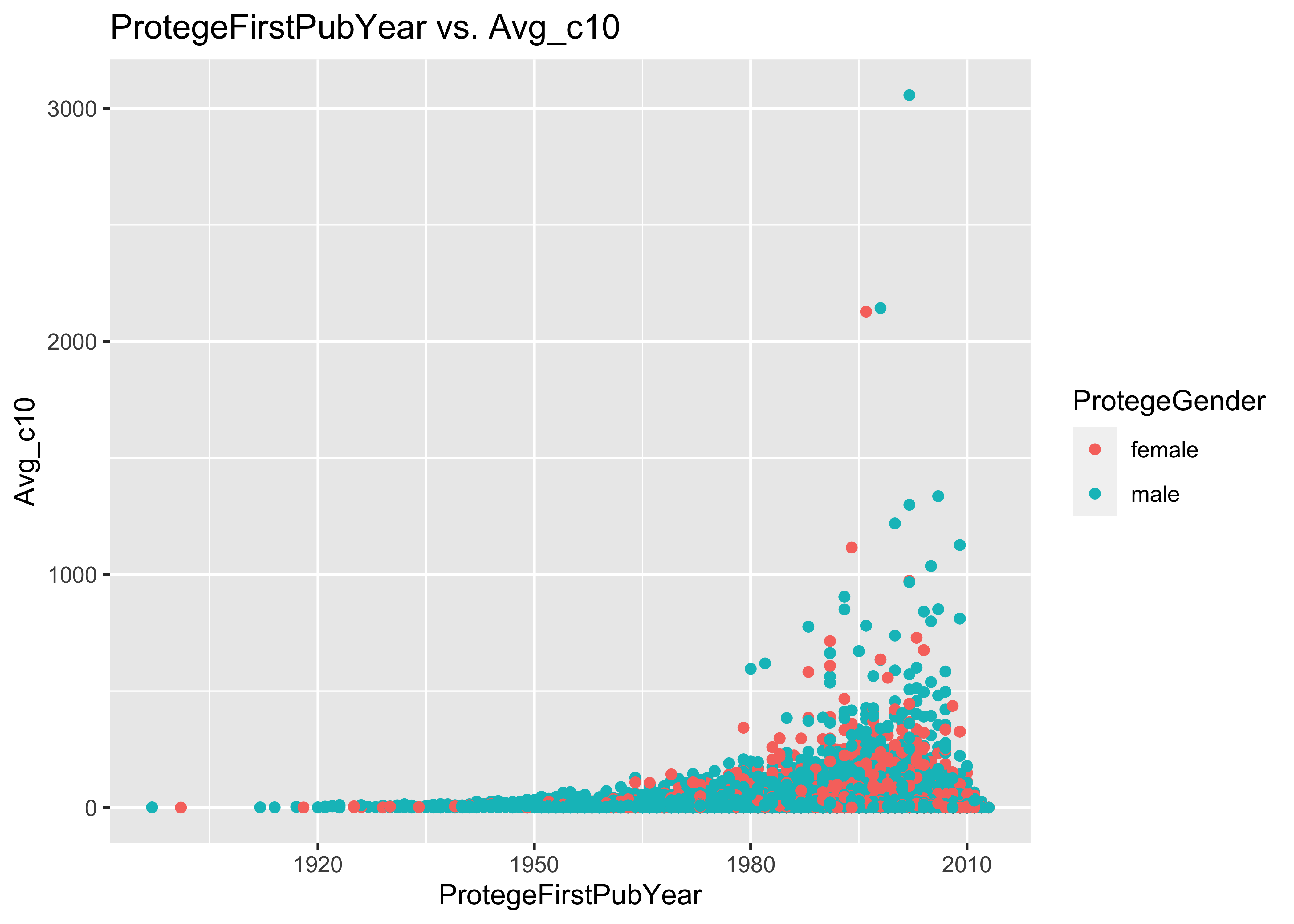
ggplot(data = a, mapping = aes(x = ProtegeFirstPubYear, y = Avg_c10, col = ProtegeGender)) +
    geom_point() + ggtitle("ProtegeFirstPubYear vs. Avg_c10")
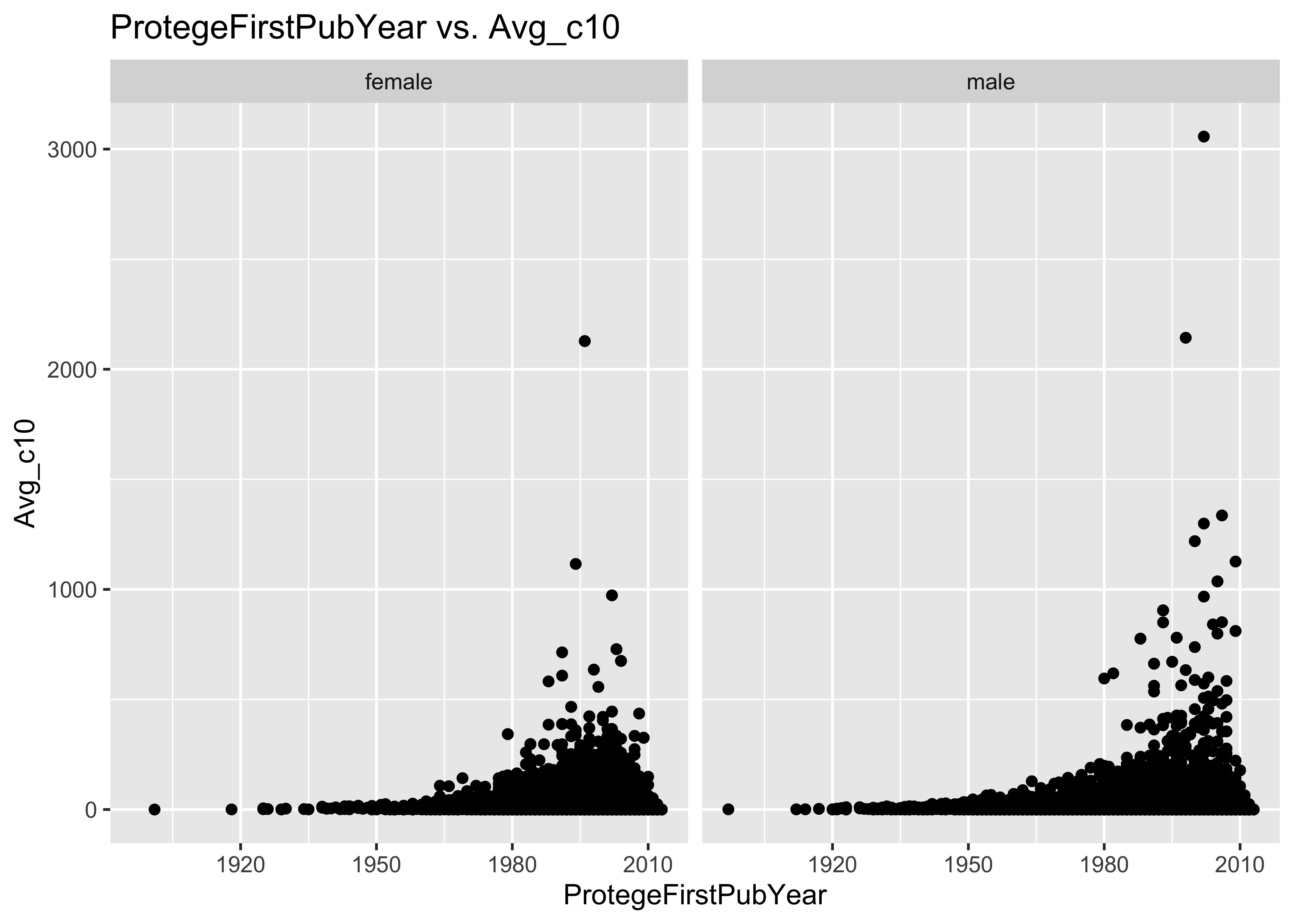
ggplot(data = a, mapping = aes(x = ProtegeFirstPubYear, y = Avg_c10)) + geom_point() +
    facet_grid(~ProtegeGender) + ggtitle("ProtegeFirstPubYear vs. Avg_c10")
10.2 Problem with Avg_c10: Cannot compute a value Avg_c10 for recent publications
As the dataset is up to Dec 31st 2019, how can one compute a valid Avg_c10 for someone whose first publication year was 2012 or 2013?
a %>% filter(ProtegeFirstPubYear == max(ProtegeFirstPubYear) - 1) %>% select(ProtegeFirstPubYear,
    Avg_c5, Avg_c10) %>% head(20)
## # A tibble: 20 x 3
##    ProtegeFirstPubYear Avg_c5 Avg_c10
##                  <dbl>  <dbl>   <dbl>
##  1                2012  0       0
##  2                2012  0       0
##  3                2012  0       0
##  4                2012  0.5     0.5
##  5                2012  0.5     0.5
##  6                2012  0       0
##  7                2012  0.5     0.5
##  8                2012  0.5     0.5
##  9                2012  0       0
## 10                2012  0.182   0.182
## 11                2012  0.182   0.182
## 12                2012  0.182   0.182
## 13                2012  0.2     0.2
## 14                2012  0       0
## 15                2012  0       0
## 16                2012  0       0
## 17                2012  0       0
## 18                2012  0       0
## 19                2012  0       0
## 20                2012  0       0
11 Avg_c5 vs Avg_c10
11.1 Tables of Avg_c5 and Avg_c10
my_controls <- tableby.control(test = T, total = T, numeric.stats = c("meansd", "medianq1q3",
    "range", "Nmiss2"), cat.stats = c("countpct", "Nmiss2"), stats.labels = list(meansd = "Mean (SD)",
    medianq1q3 = "Median (Q1, Q3)", range = "Min - Max", Nmiss2 = "Missing"))

my_controls2 <- tableby.control(numeric.stats = c("medianq1q3"), stats.labels = list(medianq1q3 = "Median (Q1, Q3)"))

t.test(Avg_c5 ~ ProtegeGender, data = a)
##
##  Welch Two Sample t-test
##
## data:  Avg_c5 by ProtegeGender
## t = 4.0045, df = 69256, p-value = 6.22e-05
## alternative hypothesis: true difference in means is not equal to 0
## 95 percent confidence interval:
##  0.3010699 0.8783127
## sample estimates:
## mean in group female   mean in group male
##             11.94469             11.35500
t.test(Avg_c10 ~ ProtegeGender, data = a)
##
##  Welch Two Sample t-test
##
## data:  Avg_c10 by ProtegeGender
## t = 2.6735, df = 69586, p-value = 0.007508
## alternative hypothesis: true difference in means is not equal to 0
## 95 percent confidence interval:
##  0.1643062 1.0669714
## sample estimates:
## mean in group female   mean in group male
##             17.34958             16.73394
t1 <- tableby(ProtegeGender ~ ., data = a %>% select(ProtegeGender, Avg_c5, Avg_c10))
summary(t1, title = "Table of Avg_c5 and Avg_c10 by ProtegeGender")
| female (N=34257) | male (N=65743) | Total (N=100000) | p value | |
|---|---|---|---|---|
| Avg_c5 | < 0.001 | |||
| Mean (SD) | 11.945 (22.121) | 11.355 (22.056) | 11.557 (22.080) | |
| Range | 0.000 - 1076.000 | 0.000 - 1126.429 | 0.000 - 1126.429 | |
| Avg_c10 | 0.008 | |||
| Mean (SD) | 17.350 (34.528) | 16.734 (34.614) | 16.945 (34.586) | |
| Range | 0.000 - 2128.000 | 0.000 - 3057.000 | 0.000 - 3057.000 |
Table of Avg_c5 and Avg_c10 by ProtegeGender
t1 <- tableby(ProtegeGender ~ ., data = a %>% select(ProtegeGender, Avg_c5, Avg_c10),
    control = my_controls2)
summary(t1, title = "Table of Avg_c5 and Avg_c10 by ProtegeGender")
| female (N=34257) | male (N=65743) | Total (N=100000) | p value | |
|---|---|---|---|---|
| Avg_c5 | < 0.001 | |||
| Median (Q1, Q3) | 7.000 (2.000, 15.000) | 6.565 (2.182, 13.969) | 6.692 (2.068, 14.254) | |
| Avg_c10 | 0.008 | |||
| Median (Q1, Q3) | 9.000 (2.286, 21.510) | 9.111 (2.935, 20.425) | 9.093 (2.694, 20.857) |
Table of Avg_c5 and Avg_c10 by ProtegeGender
t1 <- tableby(ProtegeGender ~ ., data = a %>% select(ProtegeGender, Avg_c5, Avg_c10),
    control = my_controls)
summary(t1, title = "Table of Avg_c5 and Avg_c10 by ProtegeGender")
| female (N=34257) | male (N=65743) | Total (N=100000) | p value | |
|---|---|---|---|---|
| Avg_c5 | < 0.001 | |||
| Mean (SD) | 11.945 (22.121) | 11.355 (22.056) | 11.557 (22.080) | |
| Median (Q1, Q3) | 7.000 (2.000, 15.000) | 6.565 (2.182, 13.969) | 6.692 (2.068, 14.254) | |
| Min - Max | 0.000 - 1076.000 | 0.000 - 1126.429 | 0.000 - 1126.429 | |
| Missing | 0 | 0 | 0 | |
| Avg_c10 | 0.008 | |||
| Mean (SD) | 17.350 (34.528) | 16.734 (34.614) | 16.945 (34.586) | |
| Median (Q1, Q3) | 9.000 (2.286, 21.510) | 9.111 (2.935, 20.425) | 9.093 (2.694, 20.857) | |
| Min - Max | 0.000 - 2128.000 | 0.000 - 3057.000 | 0.000 - 3057.000 | |
| Missing | 0 | 0 | 0 |
Table of Avg_c5 and Avg_c10 by ProtegeGender
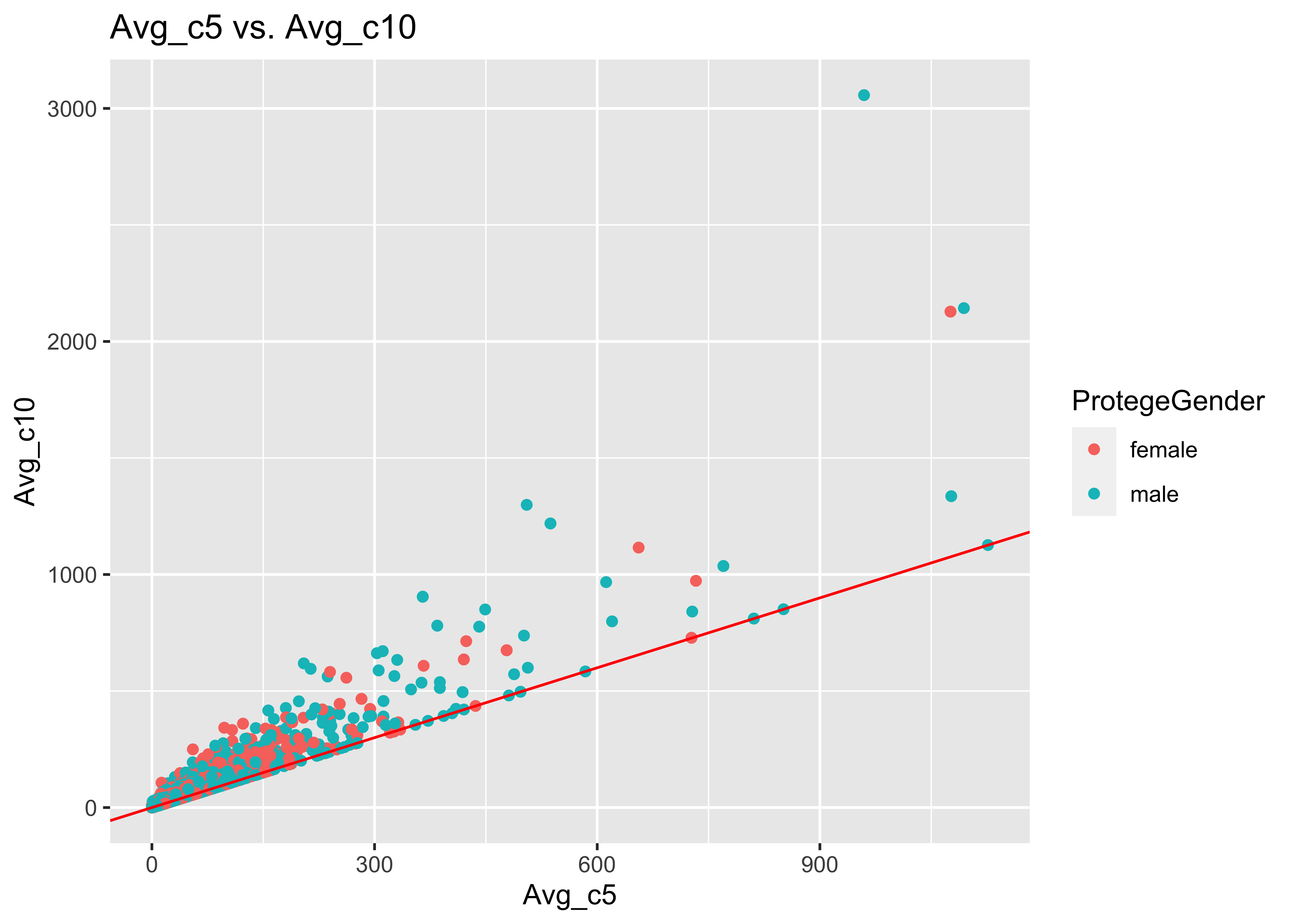
11.2 Joint distribution of Avg_c5 and Avg_c10
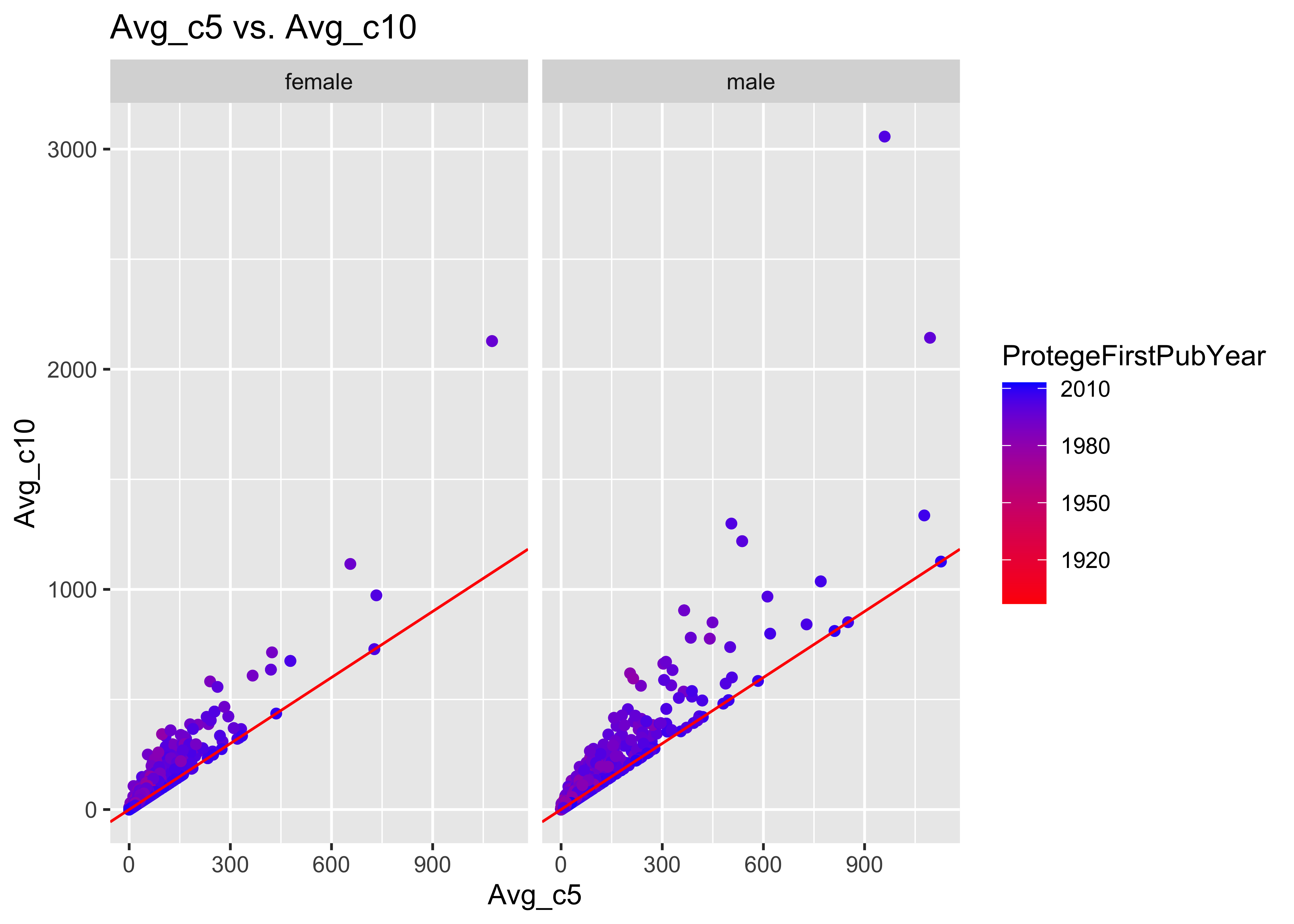
ggplot(data = a, mapping = aes(x = Avg_c5, y = Avg_c10, col = ProtegeGender)) + geom_point() +
    geom_abline(intercept = 0, slope = 1, col = "red") + ggtitle("Avg_c5 vs. Avg_c10")
ggplot(data = a, mapping = aes(x = Avg_c5, y = Avg_c10, col = ProtegeFirstPubYear)) +
    geom_point() + scale_color_gradient(low = "red", high = "blue") + geom_abline(intercept = 0,
    slope = 1, col = "red") + facet_grid(~ProtegeGender) + ggtitle("Avg_c5 vs. Avg_c10")
12 numMentors
12.1 Distribution of numMentors
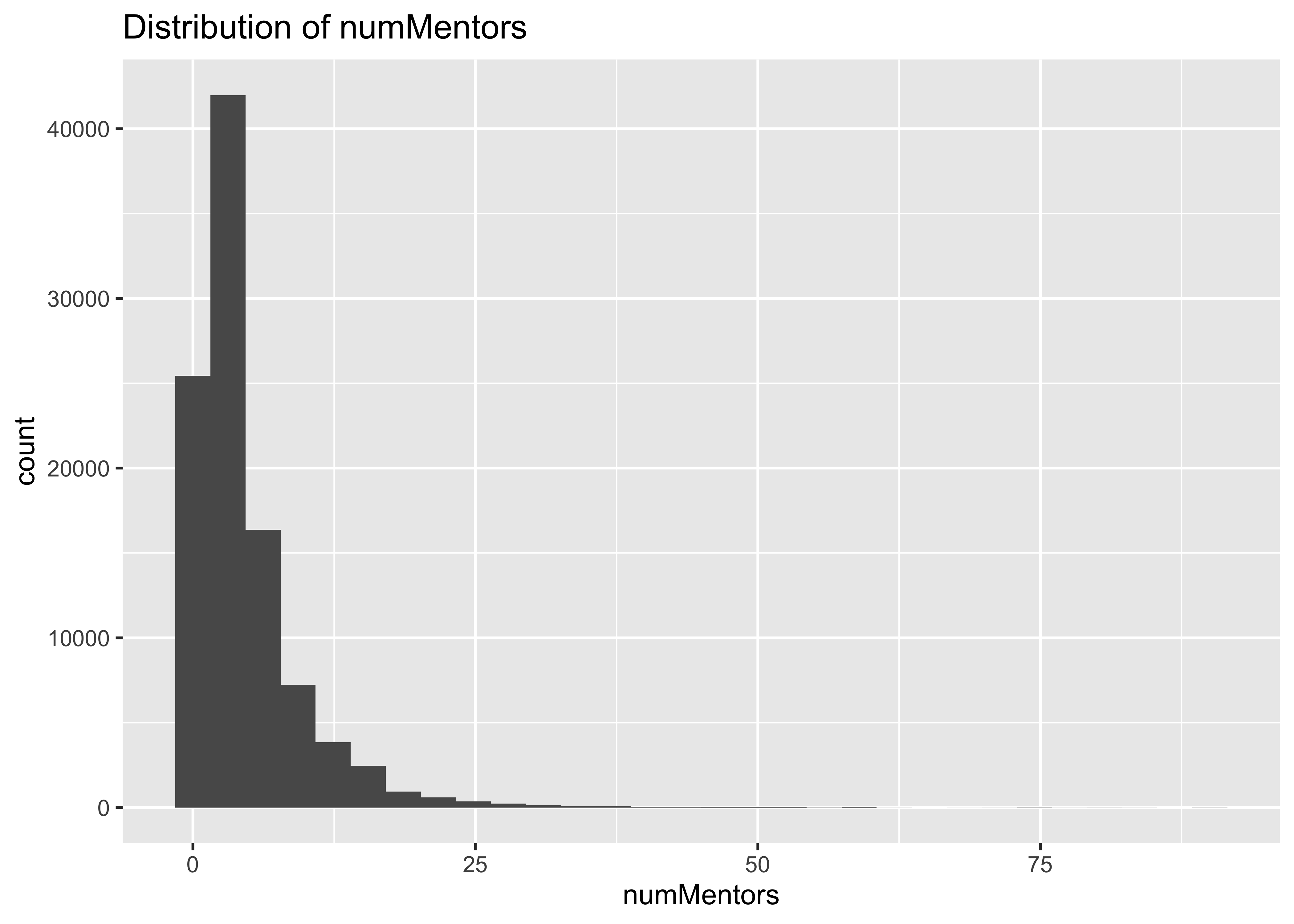
summary(a$numMentors)
##    Min. 1st Qu.  Median    Mean 3rd Qu.    Max.
##   1.000   1.000   3.000   4.514   6.000  91.000
ggplot(data = a, mapping = aes(x = numMentors)) + geom_histogram() + ggtitle("Distribution of numMentors")
## `stat_bin()` using `bins = 30`. Pick better value with `binwidth`.
ggplot(data = a, mapping = aes(x = ProtegeFirstPubYear, y = numMentors, col = ProtegeGender)) +
    geom_point() + ggtitle("ProtegeFirstPubYear vs. numMentors")
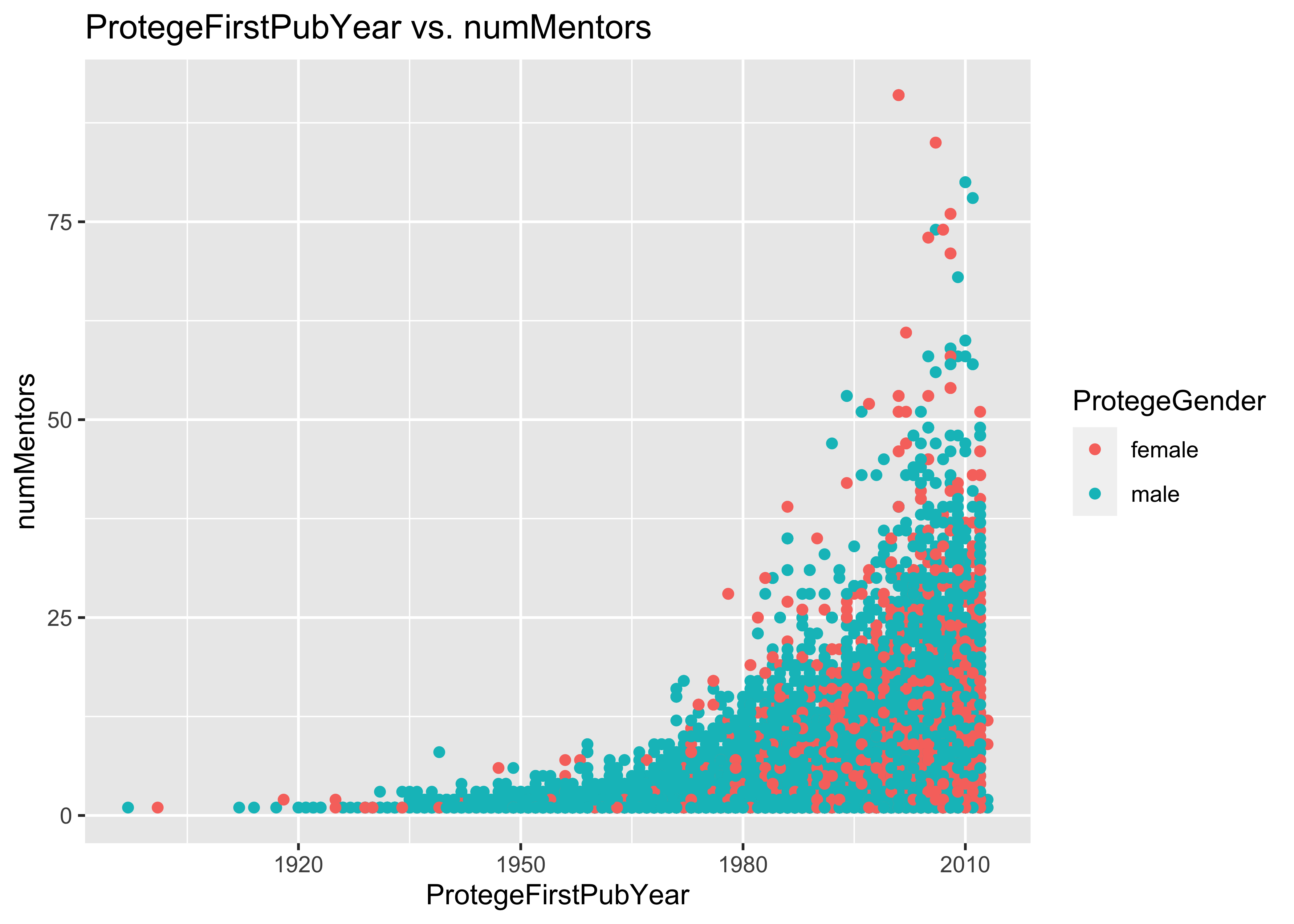
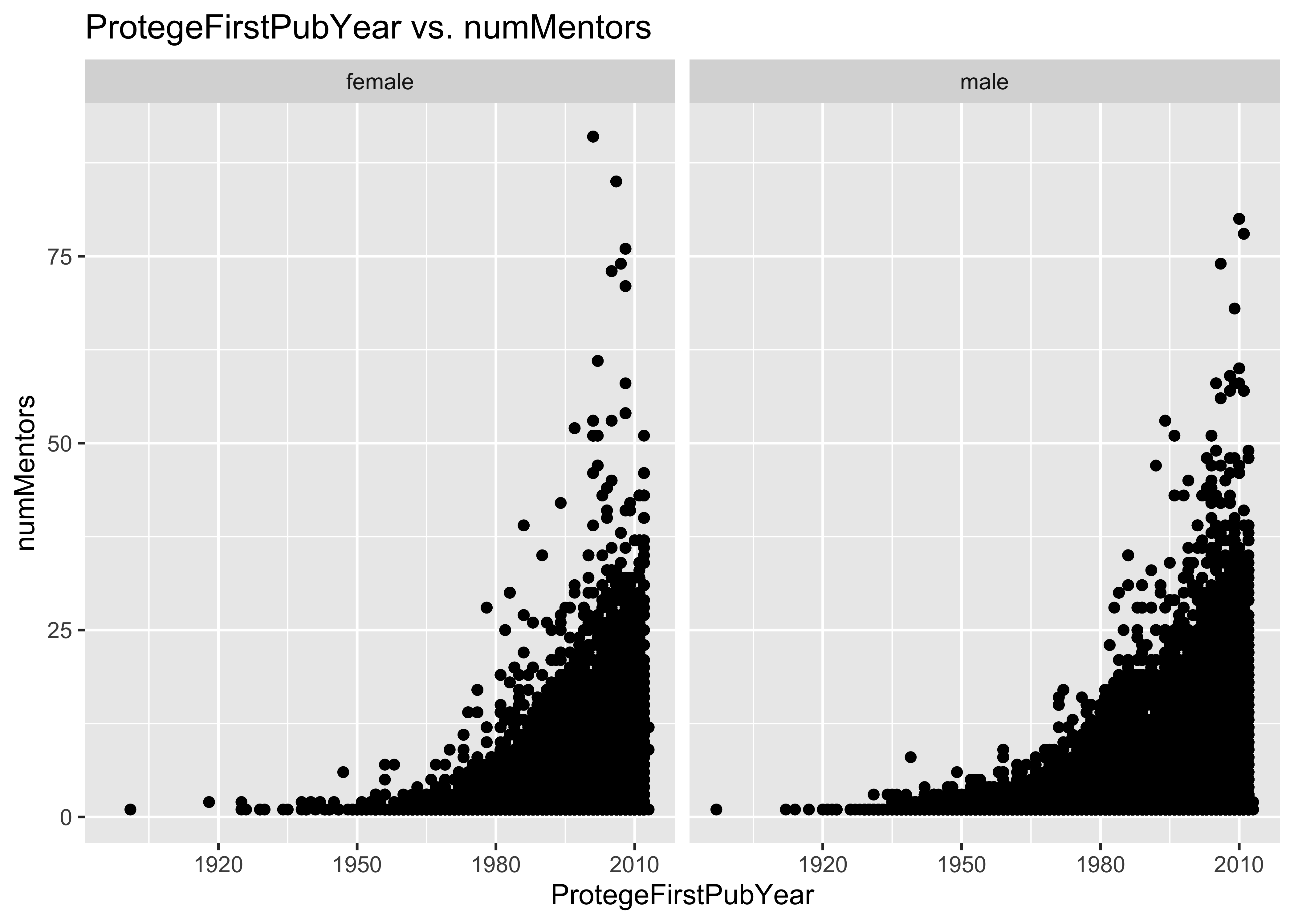
ggplot(data = a, mapping = aes(x = ProtegeFirstPubYear, y = numMentors)) + geom_point() +
    facet_grid(~ProtegeGender) + ggtitle("ProtegeFirstPubYear vs. numMentors")

12.2 Problem: some numMentors values are too large
How could someone possibly really have more than a handful of mentors?
In the first 10^{5} lines of this data set, there are individuals with 91 mentors!
The Supplement states that:
“Whenever a junior scientist publishes a paper with a senior scientist, we consider the former to be a protege, and the latter to be a mentor, as long as they authored at least one paper with 20 or less co-authors and share the same discipline and US-based affiliation.”
Oh, but we are really measuring co-authorship at the same US-based affiliation on joint papers with 20 or less co-authors.
13 Summary
Here I examine the data provided by the authors of this paper:
AlShebli B, Makovi K, Rahwan T. The association between early career informal mentorship in academic collaborations and junior author performance. Nat Commun. 2020 Nov 17;11(1):5855. doi: 10.1038/s41467-020-19723-8. PMID: 33203848. https://pubmed.ncbi.nlm.nih.gov/33203848/
For speed, I examined only the first 10^{5} lines of the data file Mentorship/Repository_Data/Data_7yearcutoff.csv from the ‘bedoor/Mentorship’ GitHub repository at
https://github.com/bedoor/Mentorship
Their repository is described by the authors as:
‘This repository includes all data used in “The Association between Early Career Informal Mentorship in Academic Collaborations and Junior Author Performance”.’
13.1 Problem: No gender information for mentors
There does not appear to be any information in the provided file about the mentor’s gender, so the provided data do not appear to be ‘all the data’.
13.2 Problem: ProtegeFirstPubYear time range is very large
In the first 10^{5} lines of this data set, the ProtegeFirstPubYear
ranges from 1897 to 2013. It seems that it would be very difficult to
properly compare the impact factors of papers published in 1897, well
before the advent of team science and the current deluge of scientific
publications, to those published as recently 2013.

13.3 Problem: Error in the equation for NumYearsPostMentorship
Note that the stated equation of 2015 - (x + 6) for computing the
number of years post mentorship is not what was used, as instead
2015 - (x + 2), where x is the year the protege’s paper was first
published.
13.4 Problem: some values of NumYearsPostMentorship are unrealistically large
In the first 10^{5} lines of the input file of this data set, there are
values of NumYearsPostMentorship as large as 116. These values are
unrealistically large.
13.5 Problem: some AvgMentorsAcAges are unrealistically large
There are AvgMentorsAcAges as large as 213 in the first 10^{5} lines
of this data set. This is unrealistically large.
Among proteges who published their first paper after 2000, there are
AvgMentorsAcAges as large as 213 in this data set. Should we be
evaluating the mentorship effects of mentors who were born than 200
years ago?
13.6 Problem with Avg_c10: Cannot compute a value Avg_c10 for recent publications
As the dataset is up to Dec 31st 2019, how can one compute a valid
Avg_c10 for someone whose first publication year was 2012 or 2013?

13.7 Problem: some numMentors values are too large
How could someone possibly really have more than a handful of mentors?
In the first 10^{5} lines of this data set, there are individuals with 91 mentors!
The Supplement states that:
“Whenever a junior scientist publishes a paper with a senior scientist, we consider the former to be a protege, and the latter to be a mentor, as long as they authored at least one paper with 20 or less co-authors and share the same discipline and US-based affiliation.”
Oh, but we are really measuring co-authorship at the same US-based affiliation on joint papers with 20 or less co-authors.
14 Generating GitHub Markdown
library(rmarkdown)
library(here)
finalize <- function() {
    rmd <- here("mentorship.Rmd")
    rmarkdown::render(rmd, "github_document")
}
15 Session Information
sessionInfo()
## R version 4.0.2 (2020-06-22)
## Platform: x86_64-apple-darwin17.0 (64-bit)
## Running under: macOS High Sierra 10.13.6
##
## Matrix products: default
## BLAS:   /System/Library/Frameworks/Accelerate.framework/Versions/A/Frameworks/vecLib.framework/Versions/A/libBLAS.dylib
## LAPACK: /Library/Frameworks/R.framework/Versions/4.0/Resources/lib/libRlapack.dylib
##
## locale:
## [1] en_US.UTF-8/en_US.UTF-8/en_US.UTF-8/C/en_US.UTF-8/en_US.UTF-8
##
## attached base packages:
## [1] stats     graphics  grDevices utils     datasets  methods
## [7] base
##
## other attached packages:
##  [1] here_0.1        rmarkdown_2.5   arsenal_3.4.0   ggExtra_0.9
##  [5] forcats_0.5.0   stringr_1.4.0   dplyr_1.0.0     purrr_0.3.4
##  [9] readr_1.3.1     tidyr_1.1.2     tibble_3.0.1    ggplot2_3.3.0
## [13] tidyverse_1.3.0 knitr_1.30
##
## loaded via a namespace (and not attached):
##  [1] Rcpp_1.0.4.6     lubridate_1.7.8  lattice_0.20-41
##  [4] utf8_1.1.4       rprojroot_1.3-2  assertthat_0.2.1
##  [7] digest_0.6.25    mime_0.9         R6_2.4.1
## [10] cellranger_1.1.0 backports_1.1.7  reprex_0.3.0
## [13] evaluate_0.14    highr_0.8        httr_1.4.2
## [16] pillar_1.4.4     rlang_0.4.6      readxl_1.3.1
## [19] rstudioapi_0.11  miniUI_0.1.1.1   Matrix_1.2-18
## [22] splines_4.0.2    labeling_0.3     munsell_0.5.0
## [25] shiny_1.5.0      broom_0.5.6      compiler_4.0.2
## [28] httpuv_1.5.4     modelr_0.1.7     xfun_0.17
## [31] pkgconfig_2.0.3  htmltools_0.5.0  tidyselect_1.1.0
## [34] fansi_0.4.1      crayon_1.3.4     dbplyr_1.4.3
## [37] withr_2.2.0      later_1.0.0      grid_4.0.2
## [40] nlme_3.1-148     jsonlite_1.6.1   xtable_1.8-4
## [43] gtable_0.3.0     lifecycle_0.2.0  DBI_1.1.0
## [46] formatR_1.7      magrittr_1.5     scales_1.1.1
## [49] cli_2.0.2        stringi_1.4.6    farver_2.0.3
## [52] fs_1.4.1         promises_1.1.0   xml2_1.3.2
## [55] ellipsis_0.3.1   generics_0.0.2   vctrs_0.3.1
## [58] tools_4.0.2      glue_1.4.1       hms_0.5.3
## [61] survival_3.1-12  fastmap_1.0.1    yaml_2.2.1
## [64] colorspace_1.4-1 rvest_0.3.5      haven_2.2.0